Prevent duplicate records in a worksheet
This article demonstrates how to set up Data Validation in order to control what the Excel user is allowed to enter. The condition is that there can't be two identical records in the Excel Table.
- Introduction
- Prevent duplicate records in a worksheet
- Prevent overlapping date and time ranges using data validation
1. Introduction
What is an Excel Table?
An Excel Table is a feature in Microsoft Excel that allows you to organize and manage data in a structured way. When you convert a range of data into a table Excel automatically applies filtering, sorting, formatting, and structured references to improve usability.
You can create a table by selecting a range of data and pressing Ctrl + T or using the "Table" button on tab "Insert" on the Ribbon.
What is Excel Data Validation?
Excel Data Validation is a feature that allows you to control what data can be entered into a cell. It helps prevent errors by restricting input based on predefined rules such as allowing only numbers, dates, or values from a list.
You can find this feature under: Tab "Data" on the ribbon. → "Data Validation" button.
What is an Excel date?
An Excel date is a numeric value representing a specific calendar day. Excel stores dates as serial numbers, where January 1, 1900 is 1, January 2, 1900 is 2, and so on. This allows for easy calculations involving dates.
What is Excel time?
An Excel time is a fractional value representing a specific time within a day. It is stored as a decimal between 0 and 1, where:
0.00 = 12:00 AM (midnight)
0.50 = 12:00 PM (noon)
0.75 = 6:00 PM
Times are fractions of a full day, so 6 hours = 0.25 (¼ of a day).
What is overlapping date and time ranges?
Overlapping date and time ranges occur when two periods partially or fully intersect. For example:
Range 1: March 1, 10:00 AM – March 1, 4:00 PM
Range 2: March 1, 2:00 PM – March 1, 6:00 PM
Since both ranges cover 2:00 PM to 4:00 PM, they overlap. Overlapping occurs when the start of one range is before the end of another, and vice versa.
2. Prevent duplicate records in a worksheet
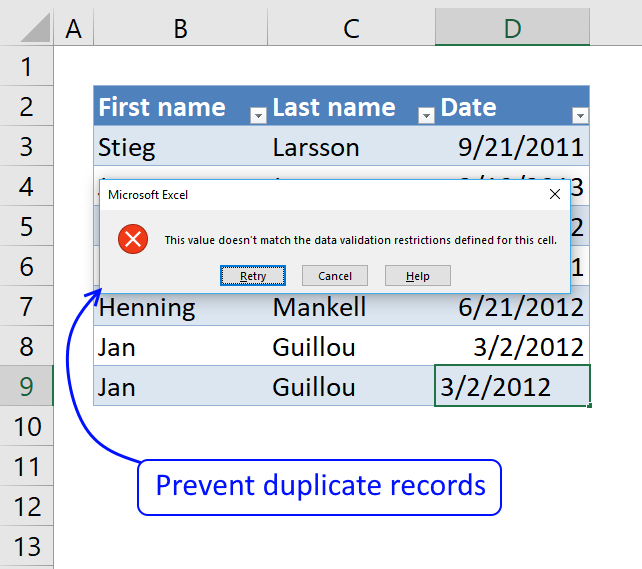
The image above shows a warning that the Excel user tried to enter a duplicate record which is not valid, the dialog box tells you that "This value doesn't match the data validation restrictions defined for this cell.
There are three buttons available, "Retry", "Cancel" and "Help" on the dialog box. The "Retry" button leaves the value as it is but selected, this allows you to edit the value you just entered. The "Cancel" button removes the value you just entered. The "Help" button opens a web page at Microsoft Support explaining how Data Validation works.
Note, it is still possible to copy and paste values to the Excel Table without the dialog box warning appearing. A green arrow in each cell corner of the record is now visible telling you that it is not valid.

Create an Excel Table

An Excel Table allows you to dynamically apply Data Validation to new data meaning if you enter a new record below the data set it will also have the same data validation rules automatically as the rest of the data.
With this setup there is no need to adjust cell ranges when new data is added or deleted, the Excel Tables does that for you instantly.
- Select any cell in the data set.
- Press shortcut keys CTRL + T to open the "Create Table" dialog box, see image above.
- Enable/disable checkbox "My table has headers" accordingly.
- Press with left mouse button on "OK" button to apply settings and create an Excel Table.

The data set is now an Excel Table which you can tell by the cell formatting and the arrows next to column headers. You can change the Excel Table style and remove "Filter" arrows next to column headers if you want.
A new tab on the ribbon named "Table Design" appears if you select on any cell in the Excel Table, it allows you to change Table Options and Styles.
Apply Data Validation
Data Validation lets you control what the Excel user can and can't enter using different methods. We are going to use a "Data Validation" formula that will trigger a dialog box warning if conditions are not met.
- Select data in your Excel Table, I selected cell range B3:D9.
- Go to tab "Data" on the ribbon.
- Press with left mouse button on "Data validation" button.
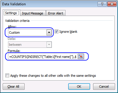
- Choose Custom, see image above.
- Type in "Formula:" field:
=COUNTIFS(INDIRECT("Table1[First name]"), $B3, INDIRECT("Table1[Last name]"), $C3, INDIRECT("Table1[Date]"), $D3)<=1
- Press with left mouse button on OK button to apply settings and create "Data Validation" to cell range B3:D8
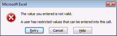
If you enter a duplicate record, the following error message appears.
Explaining the data validation formula in row 9

To learn how formulas work in greater detail I recommend the "Evaluate Formula" tool which is built-in to Excel, you can use this tool for "Data Validation" formulas as well. Copy the "Data Validation" formula and paste to a cell.
I pasted the formula to cell F3 and then pressed Enter. Select cell F3, press with left mouse button on tab "Formulas" on the ribbon. Press with left mouse button on "Evaluate Formulas" button to show the "Evaluate Formula" dialog box, see image above.
The INDIRECT function is a volatile function meaning it recalculates every time Excel recalculates, this may make it more cpu-intensive if used extensively. This function is needed in order to reference values to an Excel Table in a Data Validation formula.
This is why you get the warning text "A function in this formula causes the result to change each time the spreadsheet is calculated. The final evaluation step will match the result in the cell, but interim steps may not" in the "Evaluate Formula" dialog box, see image above.
Underlined expressions are what is about to be evaluated in the next step and italic values are the result. Press with left mouse button on the "Evaluate" button to move to the next calculation step in the formula. Press with left mouse button on "Close" button to dismiss the dialog box.
Step 1 - How to reference values in Excel data validation formulas
You can't reference Excel Tables in Data Validation formulas, however, there is a workaround. The INDIRECT function allows you to reference Excel Tables.
References to Excel Tables are called "structured references" and they don't change when values or records are added or deleted in the Excel Table.
Table1[First name]
becomes
INDIRECT("Table1[First name]")
The downside is that you need to change the formulas if you change the Table name or the Table header names accordingly, they do not change automatically in this case.
Step 2 - Count how many times a record exists in a table
The COUNTIFS function lets you count cells based on multiple conditions, we are going to count rows based on the values the Excel user enters in the Excel Table.
COUNTIFS(criteria_range1, criteria1, [criteria_range2, criteria2]…)
We will use as many criteria pairs (ranges and criteria) as there are columns in the Excel Table. I will use six arguments as there are three columns in my Excel Table. You need to adjust that to your specific Excel Table.
COUNTIFS(INDIRECT("Table1[First name]"), $B3, INDIRECT("Table1[Last name]"), $C3, INDIRECT("Table1[Date]"), $D3)
becomes
COUNTIFS($B$3:$B$9, $B3, $C$3:$C$9, $C3, $C$3:$D$9, $D3)
becomes
COUNTIFS({"Stieg"; "Jonas"; "Camilla"; "Lars"; "Henning"; "Jan"}, $B3, {"Larsson"; "Jonasson"; "Läckberg"; "Kepler"; "Mankell"; "Guillou"}, $C3, {40807; 41324; 41215; 40777; 41081; 40970}, $D3)
becomes
COUNTIFS({"Stieg"; "Jonas"; "Camilla"; "Lars"; "Henning"; "Jan" ; "Stieg"}, "Stieg", {"Larsson"; "Jonasson"; "Läckberg"; "Kepler"; "Mankell"; "Guillou"; "Larsson"}, "Larsson", {40807; 41324; 41215; 40777; 41081; 40970; 40807}, 40807)
and returns 1 in cell F3.
Step 3 - Check if number is smaller than or equal to 1
The less than sign and the equal sign together means that the number must be equal to or less than 1 in order to return True.
COUNTIFS(INDIRECT("Table1[First name]"), $B3, INDIRECT("Table1[Last name]"), $C3, INDIRECT("Table1[Date]"), $D3)<=1
becomes
1<=1
and returns TRU. The "Data validation" error message does not appear.
Recommended articles
3. Prevent overlapping date and time ranges using data validation

The picture above shows an Excel Table with Data Validation applied. An error dialog box appears if a user tries to enter an overlapping date and time range.
The image above shows an error dialog box that showed up because the date range 1/2/12 12:00 PM - 1/2/12 3:00 PM overlaps 1/2/12 11:00 AM - 1/2/12 1:00 PM.
Both the start and end of the date range must be entered to trigger the error dialog box provided the ranges overlap.
Data Validation is a feature in Excel that allows you to check values entered in your worksheet, this webpage explains it in great detail: What is Data Validation?
I am going to show you how to use a Data Validation formula in this article that checks date ranges and will warn the user if the date ranges overlap.
Create Data Validation with a custom formula
If you apply Data Validation to an Excel defined Table, all new values you enter below the last value in the Excel Table will have the same Data Validation setting applied.
In other word, the Excel table copies the Data Validation automatically to new cells when the Excel Table grows which is great and saves you time.
- Select all values except the headers in the Excel Table.
- Go to tab "Data" on the ribbon.
- Press with left mouse button on "Data Validation" button.

- Press with left mouse button on the drop-down list below "Allow:" and select "Custom", see image above.
- Type or copy/paste the following formula:
=SUMPRODUCT((INDIRECT("Table1[@Start]")<=INDIRECT("Table1[End]"))* (INDIRECT("Table1[@End]")>=INDIRECT("Table1[Start]")))<=1
- Press with left mouse button on OK button to apply Data Validation.
To be able to use Excel defined Tables in Data Validation formulas you have a few options which I have described in this article: How to use an Excel Table name in Data Validation Lists and Conditional Formatting formulas
One workaround demonstrated in the article is to use the INDIRECT function each time you reference an Excel Table, I will now explain the formula in great detail.
Explaining Data Validation formula in cell C5

A great feature with Excel Tables is that a reference pointing to an Excel Table doesn't change (unless you change the Excel Table name or headers) even if the Table grows or shrinks, the reference stays the same.
By the way, they are called structured references and they behave differently than regular cell references.
If you want to see each calculation step using the Evaluate Formula tool then copy the formula and paste to any empty cell not adjacent to the Excel Table, we will delete it later on.

Go to tab "Formula" on the ribbon and press with left mouse button on the "Evaluate Formula" button, this opens a dialog box that allows you to see each step in the calculation.
Simply press with left mouse button on the Evaluate button located on the dialog box to go to next step, keep press with left mouse button oning to see all calculation steps.
Step 1 - Check if start date is smaller than or equal to the end dates
Table1[@Start] is a reference to a cell on the same row as the selected cell and in column Start in Table1.
The less than sign and the equal sign combined checks if the value in the cell described above is less than or equal to the value in column End in Table1.
The less than and equal sign are logical operators and return a boolean value TRUE or FALSE. Table1[@Start] is a reference to a cell in column Start that is located on the same row as the current cell, in this case, cell C5. The @ character in Table1[@Start] means it is on the same row as the selected cell.
An Excel date is actually a number formatted as a date, 1/1/1900 is 1 and 1/1/2000 is 36526. There are 36525 days between 1/1/1900 and 1/1/2000.
Time is a fraction of a day, one hour is 1/24 and is approx. 0.041667 and 24 hours is 1. 12:00 PM is 0.5.
INDIRECT("Table1[@Start]")<=INDIRECT("Table1[End]")
becomes
"1/2/2012 12:00 PM"<={"1/1/12 12:00 PM", "1/2/12 1:00 PM", "1/2/12 3:00 PM"}
becomes
40910.5<={40909.5; 40910.5416666667; 40910.625}
and returns {FALSE; TRUE; TRUE}.
Step 2 - Check if end date is larger than or equal to the start dates
INDIRECT("Table1[@End]")>=INDIRECT("Table1[Start]")
becomes
"1/2/2012">={"1/1/12 8:00 AM", "1/2/12 11:00 AM", "1/2/12 12:00 PM"}
becomes
40910.625>={40909.3333333333; 40910.4583333333; 40910.5}
and returns {TRUE; TRUE; TRUE}.
Step 3 - Apply AND logic and sum array
The parentheses let you control the order of calculations, the asterisk multiplies the arrays which means that we apply AND logic meaning both values on the same row must return TRUE in order to return TRUE.
When you multiply boolean values Excel converts the output to their numerical equivalents, TRUE = 1 and FALSE = 0 (zero).
SUMPRODUCT((INDIRECT("Table1[@Start]")<=INDIRECT("Table1[End]"))* (INDIRECT("Table1[@End]")>=INDIRECT("Table1[Start]")))
becomes
SUMPRODUCT({FALSE; TRUE; TRUE}*{TRUE; TRUE; TRUE})
becomes
SUMPRODUCT({0; 1; 1})
and returns 2.
Step 4 - Check if value is less or equal to 1
If the number returned from the SUMPRODUCT function is larger than 1 we know that there is an overlapping date range.
The formula compares all ranges so the range we entered is also calculated, this makes the formula always return 1 for that row. That is why we need to check if the value is greater than 1.
SUMPRODUCT((INDIRECT("Table1[@Start]")<=INDIRECT("Table1[End]"))* (INDIRECT("Table1[@End]")>=INDIRECT("Table1[Start]")))<=1
becomes
2<=1 and returns FALSE. The error dialog box is shown.
Customize Data Validation Error Alert

- Select any value in the Excel Table.
- Go to tab "Data" on the ribbon.
- Press with left mouse button on the "Data Validation" button and a dialog box appears.

- Go to tab "Error Alert", shown in the image above.
- Enter a title.
- Enter error message. You can also choose a style.
- Press with left mouse button on OK button.

Data validation category
Table of Contents Create dependent drop down lists containing unique distinct values - Excel 365 Create dependent drop down lists […]
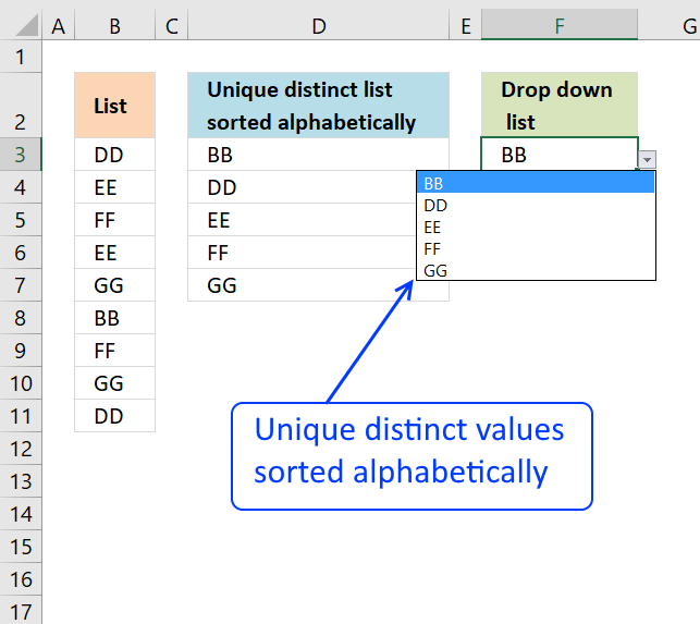
Question: How do I create a drop-down list with unique distinct alphabetically sorted values? Table of contents Introduction Sort values […]
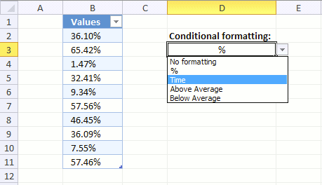
Table of contents How to change cell formatting using a Drop Down list Highlight cells based on coordinates Highlight every […]
Excel categories
2 Responses to “Prevent duplicate records in a worksheet”
Leave a Reply
How to comment
How to add a formula to your comment
<code>Insert your formula here.</code>
Convert less than and larger than signs
Use html character entities instead of less than and larger than signs.
< becomes < and > becomes >
How to add VBA code to your comment
[vb 1="vbnet" language=","]
Put your VBA code here.
[/vb]
How to add a picture to your comment:
Upload picture to postimage.org or imgur
Paste image link to your comment.
thanks for this post. I find COUNTIFS command which is very usefull.
Nice use of Indirect function to get table column data.
When we can the data from one cell to another cell then it allows the duplicate entry; How can we fix it