How to use the INDIRECT function
What is the INDIRECT function?
The INDIRECT function returns the cell reference based on a text string and shows the content of that cell reference.
Table of Contents
- Syntax
- Arguments
- How to create a cell reference?
- How to create a cell reference to a worksheet name?
- VLOOKUP and INDIRECT function
- How to create a range?
- Address
- How to use the function to another workbook?
- How to create a sum?
- How to create a column number?
- How to use INDIRECT with R1C1?
- How to hardcode a cell reference?
- How to use DataValidation with the function? (Link)
- Get Excel file
1. Syntax
INDIRECT(ref_text, [a1])
2. Arguments
| ref_text | Required. A reference to a cell, a name defined as a reference, or a reference to a cell as a text string. |
| [a1] | Optional. TRUE is the default value and is evaluated to A1- style reference. FALSE represents R1C1-style reference. |
A volatile function recalculates more often than non-volatile Excel functions, this may cause heavy CPU-usage.
Other volatile Excel functions are: OFFSET | TODAY | NOW among others.
Conditional Formatting is super-volatile, it even recalculates if you are scrolling through data.
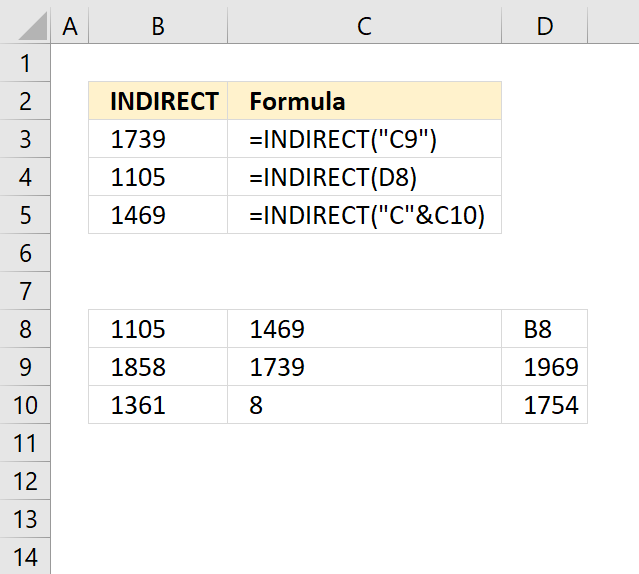
1. How to create a cell reference?

The image above demonstrates a formula in cell B8 that uses a value in cell C8 to create a cell reference.
Formula in cell B8:
1.1 Explaining formula in cell B8
Step 1 - Get value from cell
C8 returns "B3"
Step 2 - Create cell reference
INDIRECT(C8)
becomes
INDIRECT("B3")
and returns the value from cell B3 which is 2. See image above.
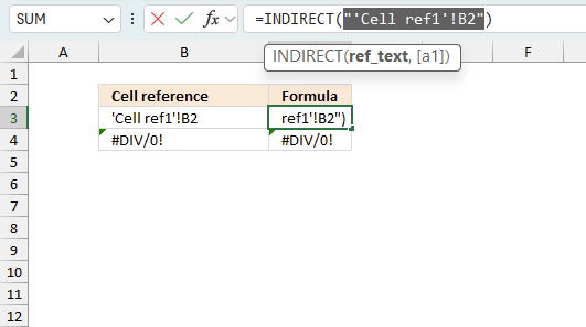
2. How to use a worksheet name?

The image above shows a formula in cell D3 that returns a value based on a worksheet name specified in cell B3 and a cell reference specified in cell C3.
Formula in cell D3:
2.1 Explaining formula in cell D3
Step 1 - Add quotes before and after worksheet name
The quotes are needed if there is a space character in the worksheet name.
"'"&B3&"'"
becomes
"'"&"Cell ref"&"'"
and returns
'Cell ref'
Step 2 - Add exclamation mark
The exclamation mark is used between the worksheet name and the cell reference.
"'"&B3&"'"&"!"
becomes
'Cell ref'&"!"
and returns
'Cell ref'!
Step 3 - Add cell reference
The cell reference i sin cell C3.
"'"&B3&"'"&"!"&C3
becomes
'Cell ref'!&C3
and returns
'Cell ref'!B2
Step 4 - Return value
INDIRECT("'"&B3&"'"&"!"&C3)
becomes
INDIRECT('Cell ref'!B2)
and returns the value from cell B2 in worksheet Cell ref.
3. VLOOKUP and INDIRECT function

The formula in cell D8, shown in the image above, contains a VLOOKUP function that uses the cell reference specified in cell B8 and a lookup value specified in cell C8 to return the correct value.
Formula in cell D8:
3.1 Explaining formula in cell D8
Step 1 - Create cell reference
INDIRECT(B8)
becomes
INDIRECT("B3:D5")
and returns
$B$3:$D$5
Step 2 - Evaluate VLOOKUP function
VLOOKUP(C8, INDIRECT(B8), 3)
becomes
VLOOKUP(C8, $B$3:$D$5, 3)
becomes
VLOOKUP(3, {1, "Blue", 5; 2, "Red", 3; 3, "Green", 4}, 3)
and returns 4.
4. How to use a range?
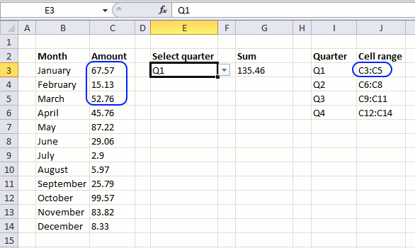
The drop-down list in cell E3 lets you select a quarter, see the animated image above. The formula in cell G3 sums the corresponding values.
Formula in cell G3:
4.1 Explaining formula in cell
Step 1 - Find relative position
The MATCH function returns the relative position of an item in an array or cell range that matches a specified value in a specific order.
MATCH(E3,I3:I6,0)
becomes
MATCH("Q1", {"Q1";"Q2";"Q3";"Q4"},0)
and returns 1.
Step 2 - Get value
The INDEX function returns a value from a cell range, you specify which value based on a row and column number.
INDEX($J$3:$J$6, MATCH(E3, I3:I6,0))
becomes
INDEX($J$3:$J$6, 1)
becomes
INDEX({"C3:C5"; "C6:C8"; "C9:C11"; "C12:C14"}, 1)
and returns "C3:C5".
Step 3 - Create cell reference
INDIRECT(INDEX($J$3:$J$6, MATCH(E3, I3:I6,0)))
becomes
INDIRECT("C3:C5")
and returns {67.57; 15.13; 52.76}
Step 4 - Sum values
The SUM function adds numbers and returns a total.
SUM(INDIRECT(INDEX($J$3:$J$6, MATCH(E3, I3:I6, 0))))
becomes
SUM({67.57; 15.13; 52.76})
and returns 135.46.
5. INDIRECT and ADDRESS function?

The formula in cell E4 gets the column number from cell E2 and the row number from E3 and creates an address to a cell.
Formula in cell E4:
5.1 Explaining formula in cell
Step 1 - Create cell address
The ADDRESS function returns the address of a specific cell, you need to provide a row and column number.
ADDRESS(row_num, column_num, [abs_num], [a1], [sheet_text])
ADDRESS(E3, E2)
becomes
ADDRESS(2, 4)
and returns $B$4
Step 2 - Get value from cell
INDIRECT(ADDRESS(E3, E2))
becomes
INDIRECT("$B$4")
and returns "B" to cell E4.
6. How to use another workbook?

The formula in cell E4 gets the column number from cell E2 and the row number from E3 and creates an address to a cell.
Formula in cell F3:
6.1 Explaining formula in cell
Step 1 - Concatenate path, workbook name and worksheet
The ampersand character lets you concatenate values.
B3&C3&D3
becomes
"C:\temp\"&"[Sales 2017.xlsx]"&"Sheet3"
and returns
"C:\temp\[Sales 2017.xlsx]Sheet3"
Step 2 - Concatenate exclamation mark and single quotes
"'"&B3&C3&D3&"'!"
becomes
"'"&"C:\temp\[Sales 2017.xlsx]Sheet3"&"'!"
and returns
"'C:\temp\[Sales 2017.xlsx]Sheet3'!"
Step 3 - Concatenate cell address
"'"&B3&C3&D3&"'!"&E3
becomes
"'C:\temp\[Sales 2017.xlsx]Sheet3'!"&E3
and returns
"'C:\temp\[Sales 2017.xlsx]Sheet3'!$B$1"
Step 4 - Create cell reference
INDIRECT("'"&B3&C3&D3&"'!"&E3)
becomes
INDIRECT("'C:\temp\[Sales 2017.xlsx]Sheet3'!$B$1")
and returns 0.6374.
7. How to create a sum?
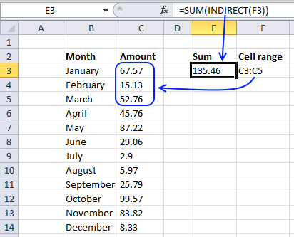
The image above demonstrates a formula in cell E3 that uses the specified cell range in F3 to sum values.
Formula in cell E3:
Cell A1 contains C3:C5. Sum function sums values in cell C3:C5. If you change the value in cell F3 to C3:C6 it sums the values in cell range C3:C6.
8. How to use a column number?

The formula in cell C8 creates a cell reference based on the specified number in cell B8.
Formula in cell F3:
8.1 Explaining formula in cell C8
Step 1 - Create an address
The ADDRESS function ceturns the address of a specific cell, you need to provide a row and column number.
ADDRESS(row_num, column_num, [abs_num], [a1], [sheet_text])
ADDRESS(1, B8, 4)
becomes
ADDRESS(1, 2, 4)
and returns "B1".
Step 2 - Calculate string length
The LEN function counts the number of characters in a given string.
LEN(ADDRESS(1, B8, 4))-1
becomes
LEN("B1")-1
becomes
2-1
and returns 1.
Step 3 - Extract column letter from address
The LEFT function extracts a specific number of characters always starting from the left.
LEFT(text, [num_chars])
LEFT(ADDRESS(1, B8, 4), LEN(ADDRESS(1, B8, 4))-1)
becomes
LEFT("B1", 1)
and returns "B".
Step 4 - Create cell reference
INDIRECT(LEFT(ADDRESS(1, B8, 4), LEN(ADDRESS(1, B8, 4))-1)&3)
becomes
INDIRECT("B"&3)
becomes
INDIRECT("B3")
and returns 0.5.
You can also use the R1C1 system to create a cell reference to a column number, see the next section below.
9. How to use R1C1?

The formula in cell D8
Formula in cell D8 :
9.1 Explaining formula in cell C8
Step 1 - Concatenate strings
The ampersand character lets you concatenate values.
"R"&B8&"C"&C8
becomes
"R"&4&"C"&2
and returns R4C2.
Step 2 - Create cell reference
The INDIRECT function has the following arguments: INDIRECT(ref_text, [a1])
[a1] stands for the style reference. TRUE is the default value and is evaluated to A1-style reference. FALSE represents R1C1-style reference.
INDIRECT("R"&B8&"C"&C8,FALSE)
becomes
INDIRECT("R4C2",FALSE)
and returns 0.3 or the value from cell B4. Cell B4 is the intersection between column 2 and row 4.
10. How to hardcode a cell reference?
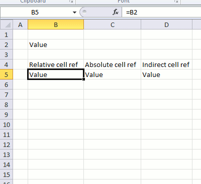
When you insert or delete a row or column in excel the cell references in formulas change, even if you use absolute cell references.
The Indirect function helps you solve that problem. The animated picture above demonstrates what happens with relative, absolute, and indirect cell references when you insert a row.
11. Function not working
The INDIRECT function returns
- ##REF! error if you use an invalid cell reference.
- #NAME? error if you misspell the function name.
- propagates errors, meaning that if the input contains an error (e.g., #VALUE!, #REF!), the function will return the same error.
11.1 Troubleshooting the error value
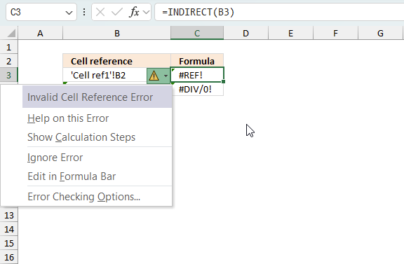
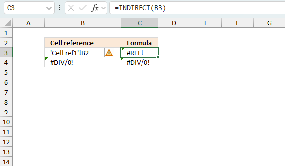
When you encounter an error value in a cell a warning symbol appears, displayed in the image above. Press with mouse on it to see a pop-up menu that lets you get more information about the error.
- The first line describes the error if you press with left mouse button on it.
- The second line opens a pane that explains the error in greater detail.
- The third line takes you to the "Evaluate Formula" tool, a dialog box appears allowing you to examine the formula in greater detail.
- This line lets you ignore the error value meaning the warning icon disappears, however, the error is still in the cell.
- The fifth line lets you edit the formula in the Formula bar.
- The sixth line opens the Excel settings so you can adjust the Error Checking Options.
Here are a few of the most common Excel errors you may encounter.
#NULL error - This error occurs most often if you by mistake use a space character in a formula where it shouldn't be. Excel interprets a space character as an intersection operator. If the ranges don't intersect an #NULL error is returned. The #NULL! error occurs when a formula attempts to calculate the intersection of two ranges that do not actually intersect. This can happen when the wrong range operator is used in the formula, or when the intersection operator (represented by a space character) is used between two ranges that do not overlap. To fix this error double check that the ranges referenced in the formula that use the intersection operator actually have cells in common.
#SPILL error - The #SPILL! error occurs only in version Excel 365 and is caused by a dynamic array being to large, meaning there are cells below and/or to the right that are not empty. This prevents the dynamic array formula expanding into new empty cells.
#DIV/0 error - This error happens if you try to divide a number by 0 (zero) or a value that equates to zero which is not possible mathematically.
#VALUE error - The #VALUE error occurs when a formula has a value that is of the wrong data type. Such as text where a number is expected or when dates are evaluated as text.
#REF error - The #REF error happens when a cell reference is invalid. This can happen if a cell is deleted that is referenced by a formula.
#NAME error - The #NAME error happens if you misspelled a function or a named range.
#NUM error - The #NUM error shows up when you try to use invalid numeric values in formulas, like square root of a negative number.
#N/A error - The #N/A error happens when a value is not available for a formula or found in a given cell range, for example in the VLOOKUP or MATCH functions.
#GETTING_DATA error - The #GETTING_DATA error shows while external sources are loading, this can indicate a delay in fetching the data or that the external source is unavailable right now.
11.2 The formula returns an unexpected value
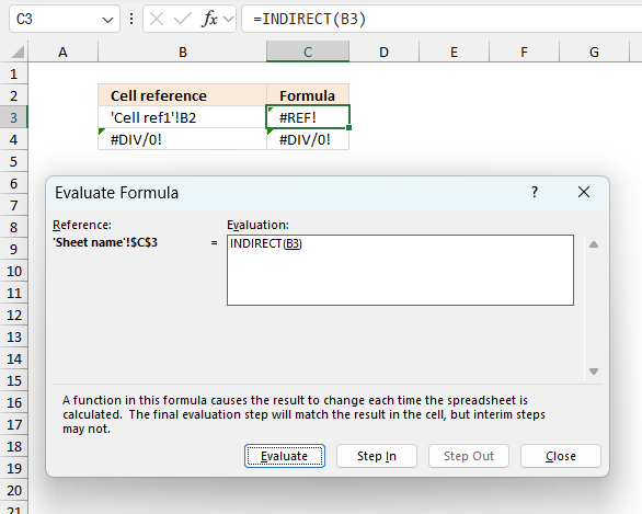
To understand why a formula returns an unexpected value we need to examine the calculations steps in detail. Luckily, Excel has a tool that is really handy in these situations. Here is how to troubleshoot a formula:
- Select the cell containing the formula you want to examine in detail.
- Go to tab “Formulas” on the ribbon.
- Press with left mouse button on "Evaluate Formula" button. A dialog box appears.
The formula appears in a white field inside the dialog box. Underlined expressions are calculations being processed in the next step. The italicized expression is the most recent result. The buttons at the bottom of the dialog box allows you to evaluate the formula in smaller calculations which you control. - Press with left mouse button on the "Evaluate" button located at the bottom of the dialog box to process the underlined expression.
- Repeat pressing the "Evaluate" button until you have seen all calculations step by step. This allows you to examine the formula in greater detail and hopefully find the culprit.
- Press "Close" button to dismiss the dialog box.
There is also another way to debug formulas using the function key F9. F9 is especially useful if you have a feeling that a specific part of the formula is the issue, this makes it faster than the "Evaluate Formula" tool since you don't need to go through all calculations to find the issue..
- Enter Edit mode: Double-press with left mouse button on the cell or press F2 to enter Edit mode for the formula.
- Select part of the formula: Highlight the specific part of the formula you want to evaluate. You can select and evaluate any part of the formula that could work as a standalone formula.
- Press F9: This will calculate and display the result of just that selected portion.
- Evaluate step-by-step: You can select and evaluate different parts of the formula to see intermediate results.
- Check for errors: This allows you to pinpoint which part of a complex formula may be causing an error.
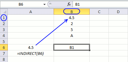
The image above shows cell reference B3 converted to hard-coded value using the F9 key. The INDIRECT function requires valid cell references which is not the case in this example. We have found what is wrong with the formula.
Tips!
- View actual values: Selecting a cell reference and pressing F9 will show the actual values in those cells.
- Exit safely: Press Esc to exit Edit mode without changing the formula. Don't press Enter, as that would replace the formula part with the calculated value.
- Full recalculation: Pressing F9 outside of Edit mode will recalculate all formulas in the workbook.
Remember to be careful not to accidentally overwrite parts of your formula when using F9. Always exit with Esc rather than Enter to preserve the original formula. However, if you make a mistake overwriting the formula it is not the end of the world. You can “undo” the action by pressing keyboard shortcut keys CTRL + z or pressing the “Undo” button
11.3 Other errors
Floating-point arithmetic may give inaccurate results in Excel - Article
Floating-point errors are usually very small, often beyond the 15th decimal place, and in most cases don't affect calculations significantly.
Useful links
INDIRECT function - Microsoft
How to use INDIRECT function in Excel - formula examples
'INDIRECT' function examples
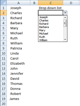
Table of Contents Add values to a regular drop-down list programmatically How to insert a regular drop-down list Add values […]
Table of contents How to change cell formatting using a Drop Down list Highlight cells based on coordinates Highlight every […]
Table of Contents Excel monthly calendar - VBA Calendar Drop down lists Headers Calculating dates (formula) Conditional formatting Today Dates […]
Functions in 'Lookup and reference' category
The INDIRECT function function is one of 25 functions in the 'Lookup and reference' category.
How to comment
How to add a formula to your comment
<code>Insert your formula here.</code>
Convert less than and larger than signs
Use html character entities instead of less than and larger than signs.
< becomes < and > becomes >
How to add VBA code to your comment
[vb 1="vbnet" language=","]
Put your VBA code here.
[/vb]
How to add a picture to your comment:
Upload picture to postimage.org or imgur
Paste image link to your comment.
Contact Oscar
You can contact me through this contact form