Comparing Excel Sorting Techniques: Formulas, Tools, and VBA

I will in this article discuss three different techniques to sort a data set in Excel. I am going to compare these and present their advantages and disadvantages.
- Formulas. The first method sorts a data set using array formulas and explain in detail how the formulas work.
- Dynamic and fast. Why would you want to sort a dataset using formulas when Excel has tools built-in that works great? Formulas are dynamic and change instantly when new values are added. This is great for interactive worksheets and dashboards to make the user experience as smooth as possible, in other words, as easy it can possibly be.
- Earlier Excel formulas. Older sorting formulas in Excel were complicated and significantly limited by the functions available at the time.
- Excel 365 functions. Very easy to work with. The output refreshes immediately if changes are made. Spills to adjacent cells automatically.
- Built-in tools. Excel has built-in tools that allow you to sort data quickly and easily.
- Sort tool. Access this on tab "Data" on the ribbon. The button is named "Sort".
- Sort with right mouse button. Press with right mouse button on on the data you want to sort. A popup menu allows you to sort values.
- Excel defined Table. Has a built-in sorting. The buttons next to the column header names allows you to sort.
- Autofilter. This feature allows you to filter and sort data. The buttons next to the column header names allows you to sort.
- Sort with VBA. A macro that demonstrates what visual basic for applications is capable of.
What's on this page
1. Sort using a formula in older Excel versions

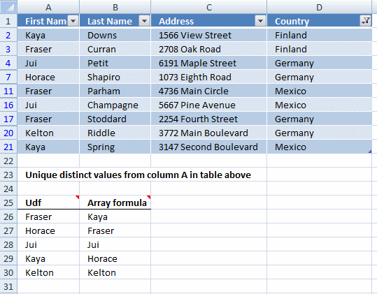
In older versions of Excel, it was quite difficult to create formulas that could sort values, as you will soon see. The image above displays a data set across three columns. To sort a three column data set required an incredible large formula. The following formula is too large to be useful:
- Hard to troubleshoot.
- Changing cell references is tedious.
- Complicated to extend formula to include more columns.
- Needs to be entered as an array formula.
- You need to extend the formula to more cells manually if the dataset grows.
Array formula in cell F3:
I recommend using the built-in options if you are working with older Excel versions than Excel 365. See section 3 for an Excel 365 formula.
How to enter an array formula
- Copy array formula.
- Select cell F3.
- Press with left mouse button on in formula bar.
- Paste array formula to formula bar.
- Press and hold CTRL + SHIFT.
- Press Enter.
How to copy array formula
- Select cell F3.
- Copy cell (Ctrl +c).
- Select cell range G:3:H3.
- Paste (Ctrl + v).
- Select cell range F3:H3.
- Copy (Ctrl + c).
- Select cell range F4:H8.
- Paste (Ctrl + v).
1.1 Explaining array formula in cell F3
Step 1 - Sort Col B from A to Z using the COUNTIF function
The COUNTIF function counts cells based on a condition, however, using a different approach with a less than sign you can create an array containing numbers representing the sort order.
The relative position of each number in the array corresponds to the same value in cell range $B$3:$B$8.
COUNTIF($B$3:$B$20, "<"&$B$3:$B$20)
becomes
COUNTIF({"A"; "A"; "A"; "A"; "A"; "A"; "A"; "A"; "A"; "A"; "A"; "A"; "A"; "A"; "A"; "A"; "A"; "A"}, {"<A";"<A";"<A";"<A";"<A";"<A";"<A";"<A";"<A";"<A";"<A";"<A";"<A";"<A";"<A";"<A";"<A";"<A"})
and returns
{0; 0; 0; 0; 0; 0; 0; 0; 0; 0; 0; 0; 0; 0; 0; 0; 0; 0}.
Step 2 - Sort Col C from A to Z with COUNTIF function
This part of the formula also creates an array containing numbers representing the sort order of each item in column C, however, it also divides the numbers with 10, 100 or 1000 etc based on the number of rows in the data set.
The ROWS function returns the number of rows in a cell range or a structured reference meaning a cell reference pointing to an Excel Table.
COUNTIF($C$3:$C$20, "<"&$C$3:$C$20)/(10^CEILING(LOG10(ROWS(Table1[Col B])), 1))
becomes
COUNTIF($C$3:$C$20, "<"&$C$3:$C$20)/(10^CEILING(LOG10(18), 1))
The next steps rounds the number to the nearest power of 10. Example, 5 returns 10. 99 returns 100. 101 returns 1000 and so on.
The LOG10 function calculates the logarithm of a number using the base 10.
COUNTIF($C$3:$C$20, "<"&$C$3:$C$20)/(10^CEILING(LOG10(18), 1))
becomes
COUNTIF($C$3:$C$20, "<"&$C$3:$C$20)/(10^CEILING(1.25527250510331, 1))
The CEILING function rounds a number up to its nearest multiple.
COUNTIF($C$3:$C$20, "<"&$C$3:$C$20)/(10^CEILING(1.25527250510331, 1))
becomes
COUNTIF($C$3:$C$20, "<"&$C$3:$C$20)/(10^2)
The ^ character works just like the POWER function, it calculates a number raised to a power.
COUNTIF($C$3:$C$20, "<"&$C$3:$C$20)/(10^2)
becomes
COUNTIF($C$3:$C$20, "<"&$C$3:$C$20)/100
and returns
{0.17; 0.16; 0.15; 0.14; 0.13; 0.12; 0.11; 0.1; 0.09; 0.08; 0.07; 0.06; 0.05; 0.04; 0.01; 0.03; 0.01; 0}.
Step 3 - Sort Col D from A to Z with COUNTIF function
Column D is the third and last column in the data set.
COUNTIF($D$3:$D$20, "<"&$D$3:$D$20)/(10^CEILING(LOG10(ROWS(Table1[Col B])), 1))^2
returns
{0; 0.0002; 0.0003; ... ; 0.0017}.
Step 4 - Add all arrays
The plus character allows you to add arrays, we have three arrays in this calculation.
COUNTIF($B$3:$B$20, "<"&$B$3:$B$20)+COUNTIF($C$3:$C$20, "<"&$C$3:$C$20)/(10^CEILING(LOG10(ROWS(Table1[Col B])), 1))+COUNTIF($D$3:$D$20, "<"&$D$3:$D$20)/(10^CEILING(LOG10(ROWS(Table1[Col B])), 1))^2
returns {0.17; 0.1602; ... ; 0.0017}.
Step 5 - Return the k-th smallest value
The SMALL function extracts the k-th smallest value from a cell range or array.
SMALL(array, k)
SMALL(COUNTIF($B$3:$B$20, "<"&$B$3:$B$20)+COUNTIF($C$3:$C$20, "<"&$C$3:$C$20)/(10^CEILING(LOG10(ROWS(Table1[Col B])), 1))+COUNTIF($D$3:$D$20, "<"&$D$3:$D$20)/(10^CEILING(LOG10(ROWS(Table1[Col B])), 1))^2, ROW(B1))
returns 0.0017
Step 6 - Find the relative position
To be able to get the correct value we need to find the position of the k-th smallest value in the array. The MATCH function returns the relative position.
MATCH(SMALL(COUNTIF($B$3:$B$8, "<"&$B$3:$B$8)+COUNTIF($C$3:$C$8, "<"&$C$3:$C$8)/10+COUNTIF($D$3:$D$8, "<"&$D$3:$D$8)/100, ROW(A1)), COUNTIF($B$3:$B$8, "<"&$B$3:$B$8)+COUNTIF($C$3:$C$8, "<"&$C$3:$C$8)/10+COUNTIF($D$3:$D$8, "<"&$D$3:$D$8)/100, 0)
returns 18.
Step 7 - Return the corresponding value
The INDEX function is able to fetch the value from a given cell range based on arow and column number.
INDEX($B$3:$D$20, MATCH(SMALL(COUNTIF($B$3:$B$20, "<"&$B$3:$B$20)+COUNTIF($C$3:$C$20, "<"&$C$3:$C$20)/(10^CEILING(LOG10(ROWS(Table1[Col B])), 1))+COUNTIF($D$3:$D$20, "<"&$D$3:$D$20)/(10^CEILING(LOG10(ROWS(Table1[Col B])), 1))^2, ROW(B1)), COUNTIF($B$3:$B$20, "<"&$B$3:$B$20)+COUNTIF($C$3:$C$20, "<"&$C$3:$C$20)/(10^CEILING(LOG10(ROWS(Table1[Col B])), 1))+COUNTIF($D$3:$D$20, "<"&$D$3:$D$20)/(10^CEILING(LOG10(ROWS(Table1[Col B])), 1))^2, 0), COLUMN(A1))
returns A in cell F3.
2. Excel 365 sort functions
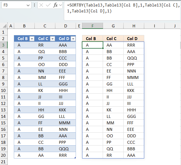
The latest version Excel 365 introduced new sorting functions that made sorting really easy to do. The SORT and SORTBY functions are an incredible addition to Excel 365.
Excel 365 dynamic array formula in cell F3:
The SORTBY function sorts a cell range or array based on values in a corresponding range or array.
Function syntax: SORTBY(array, by_array1, [sort_order1], [by_array2, sort_order2],…)
The formula in cell F3 returns the entire data set to cells below and to the right, sorted based on the arguments provided.
What is an Excel 365 dynamic array?
It is a new formula feature available only to Excel 365 subscribers:
- Spills values to adjacent cells automatically if needed. A #SPILL! error means that the destination cells are not empty (populated).
- There is no need anymore for entering array formulas as we used to do in earlier Excel versions. Simply press Enter and the Excel 365 formula will automatically spill values to adjacent cells if needed.
What is an interactive dashboard in Excel?
An interactive dashboard in Excel is a visual tool that allows users to explore and analyze data in a dynamic and engaging way. Unlike static reports, interactive dashboards enable users to manipulate data, drill down into details, and gain insights in real-time. It is often built based on:
- Interactive Buttons: Users can press with left mouse button on buttons (created using Form Controls or ActiveX) directly on the worksheet to trigger actions and automate various tasks within the dashboard.
- Real-time Formula Updates: Dynamic formulas ensure that the dashboard instantly reflects any changes made by the user, providing immediate feedback and up-to-date analysis.
- Simplified Input with Drop-Down Lists: Drop-down lists offer a user-friendly way to input data and control values, ensuring data accuracy and ease of interaction.
- Data Visualization through Charts: Charts are used to visually represent data, enabling users to analyze trends, patterns, and insights quickly and effectively.
Why use an Excel Table?
Excel tables offer a significant advantage for interactive dashboards: a cell reference to an Excel Table automatically adjust when data is added or removed. This dynamic referencing ensures the dashboard remains user-friendly and requires no manual updates when the underlying data changes.
Why use an Excel 365 formula combined with an Excel Table that already sorts values automatically?
The Excel Table does sort the values but not automatically. The user needs to sort the values again if new values are added or deleted by interacting with the buttons next to the column header names.
What is the main disadvantage with dynamic array formulas?
An older computer may have problems returning a really large sorted dataset. This is obvious if the calculation takes time or Excel freezes while calculating.
3. Sort using the built-in "Sort" feature

For users of interactive Excel worksheets or dashboards with form controls, ActiveX controls, or drop-down lists linked to data, manually sorting values using Excel's built-in features can be problematic. Even with these tools, repeatedly sorting data whenever conditions change or new data is added can become tedious and time-consuming, detracting from the user experience.
Why is using the SORT tool considered manual work?
The SORT tool does not require manually moving values, but applying it to a dataset initially involves manual effort. After the first application, sorting can be adjusted with minimal interaction using the buttons next to the column headers. However, sorting must be reapplied each time the source data changes. In contrast, dynamic array formulas or VBA with event-driven code can automate this process.
Where is the SORT tool?
The SORT tool is accessible as a button on the "Data" tab on the ribbon. You can also use Excel's Sort feature which is located on the "Home" tab on the ribbon.
How to enable the SORT tool?
Follow these steps:
- Select the entire data set including the header names.
- Go to tab "Home" on the ribbon.
- Press with mouse on the "Sort & Filter" button.
- Press with mouse on "Custom Sort..." and a dialog box appears.

- Sort the first column by column B.

- Press with mouse on "Add Level" button.

- Sort the second column by column C.

- Press with mouse on "Add Level" button.
- Sort the third column by column D.

- Press with left mouse button on the OK button to apply changes.
Tip! Press with mouse on "A to Z" to change the sort order from "A to Z" to "Z to A". Disable checkbox "My data has headers" if your data set has no column names.
4. Sort using VBA

This example demonstrates a button that is linked to a macro, press with left mouse button on the button to start the macro. I will also show you how to run the macro if a cell on the same worksheet has been changed using event code.
The last technique I will demonstrate is to use a macro that sorts values based on certain conditions like if a value is changed or a worksheet is activated etc, it is event code that makes this possible. They are not placed on the same module as regular macros but in worksheet or workbook modules which I will also describe in detail in this article.
What is VBA?
VBA (Visual Basic for Applications) is a programming language developed by Microsoft that is used for automating tasks in Microsoft Office applications such as Excel, Word, and Access. It allows users to create macros, automate repetitive tasks, and enhance Office functionality with custom scripts.
How to enable developer tab?
Here is how to enable the "Developer" tab if it is missing on the ribbon:
- Press with left mouse button on "File" located above the ribbon, a new pane appears.
- Press with mouse on the "Options" button to access Excel settings.
- Press with mouse on "Customize Ribbon" and then on the right side press with left mouse button on the checkbox next to the tab "Developer" to enable it.
- Press with left mouse button on "OK" button to apply changes.
The "Developer" tab is now visible on the ribbon. Here are instructions for Excel 2007, Excel 2010 and Excel 2013
4.1 VBA code
Sub Macro1()
'Allows you to write shorter code by referring to an object only once instead of using it with each property.
With ActiveWorkbook.Worksheets("VBA").Sort

    'Clear previous sort conditions
    .SortFields.Clear

    'Apply sorting from A to Z to cell range B3:B8
    .SortFields.Add2 Key:=Range("B3:B8"), SortOn:=xlSortOnValues, Order:=xlAscending, DataOption:=xlSortNormal

    'Apply sorting from A to Z to cell range C3:C8
    .SortFields.Add2 Key:=Range("C3:C8"), SortOn:=xlSortOnValues, Order:=xlAscending, DataOption:=xlSortNormal

     'Apply sorting from A to Z to cell range D3:D8
    .SortFields.Add2 Key:=Range("D3:D8"), SortOn:=xlSortOnValues, Order:=xlAscending, DataOption:=xlSortNormal

    'Set range to B2:D8
    .SetRange Range("B2:D8")

    'Column names exists
    .Header = xlYes

    'No case sensitivity
    .MatchCase = False

    'Sort orientation xlTopToBottom vs xlLeftToRight
    .Orientation = xlTopToBottom

    'Apply sorting to range
    .Apply
End With
End Sub
4.2 Where to put the VBA code?

- Press Alt + F11 to open the Visual Basic Editor.
- Press with mouse on "Insert" on the top menu.
- Press with mouse on "Module" to insert a module to your workbook. It is named Module1 in the image above.
- Copy above VBA code.
- Paste to code window.
4.3 How to create a button linked to the macro
- Go to tab "Developer" on the ribbon.
- Press with mouse on "Insert Controls" button.
- Press with mouse on "Button" button.
- Press with left mouse button on and drag on the worksheet to create the button. You can always later resize the button.
- A dialog box appears asking for a macro to be assigned. Select the macro you want to use and press with left mouse button on OK.
What is a Form Control?
Form Controls are built-in user interface elements in Microsoft Excel and other Microsoft Office applications that allow users to interact with spreadsheets or documents. These controls include buttons, checkboxes, dropdown lists, scroll bars, and more. Form Controls are relatively simple and are linked directly to spreadsheet cells, allowing for easy data manipulation without the need for complex coding.
- Simple to use and configure.
- Work with Excel’s built-in macros and formulas.
- Do not require programming knowledge (VBA is optional).
- Faster and more lightweight compared to ActiveX controls.
- Limited customization options.
4.4 Event code

Event code allows you to run the sort macro automatically based on specific things that can happen, for instance, activating the worksheet, selecting a cell or in this case, if a cell value has changed.
What is an event?
An event in Excel refers to an action or occurrence that triggers the execution of a specific macro. Events can be user-initiated, such as opening a workbook, changing a cell's value, or press with left mouse button oning a button, or system-initiated, like recalculating a worksheet. By associating macros with events users can automate responses to specific actions within the workbook.
What is event code?
Event code is placed in specific object modules like ThisWorkbook or a worksheet module (Sheet1, Sheet2). Regular VBA code is typically stored in a standard VBA module like Module1, Module2, etc...
'Event code that is rund when a cell value in worksheet VBA changes
Private Sub Worksheet_Change(ByVal Target As Range)

'Start macro named macro1
Macro1

End Sub
4.5 Where to put the Event code?

- Press with right mouse button on on the worksheet tab located at the very bottom of your Excel Screen.
- Press with mouse on "View Code".
- The Visual Basic Editor opens with the worksheet module selected.
- Copy and paste the event code above to the worksheet module.
- Exit VB Editor and return to Excel.
Table category
Table of Contents How to compare two data sets - Excel Table and autofilter Filter shared records from two tables […]
This article demonstrates different ways to reference an Excel defined Table in a drop-down list and Conditional Formatting formulas. The […]
This article demonstrates two formulas that extract distinct values from a filtered Excel Table, one formula for Excel 365 subscribers […]
Sort values category
Table of Contents Sort a column - Excel 365 Sort a column using array formula Two columns sorting by the […]
How to use Excel Tables
One Response to “Comparing Excel Sorting Techniques: Formulas, Tools, and VBA”
Leave a Reply
How to comment
How to add a formula to your comment
<code>Insert your formula here.</code>
Convert less than and larger than signs
Use html character entities instead of less than and larger than signs.
< becomes < and > becomes >
How to add VBA code to your comment
[vb 1="vbnet" language=","]
Put your VBA code here.
[/vb]
How to add a picture to your comment:
Upload picture to postimage.org or imgur
Paste image link to your comment.
Ola,
Gostaria de fazer uma classificação de pares e impares para jogos aqui no Brasil.
Assim:
de c3 até q3000 quinze dezenas (numeros)
de U3 em diante separar Impares e Pares
Desde ja agradeço
Rogerio