Find missing numbers
Table of Contents
- Find missing numbers in a column based on a given range
- Find missing three character alpha code numbers
- Insert blank rows for missing values
- Identify missing numbers in two columns combined based on a numerical range
- Identify missing numbers in two columns combined based on a numerical range - Excel 365
1. Identify missing numbers in a column based on a given range
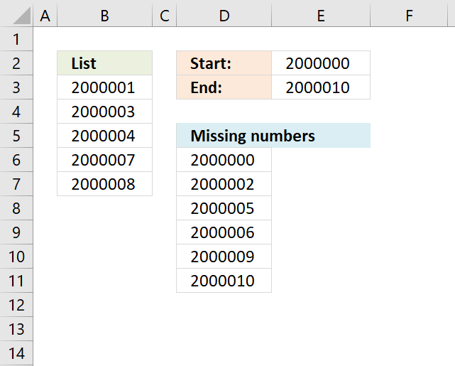
The image above shows an array formula in cell D6 that extracts missing numbers i cell range B3:B7, the lower boundary is specified in cell E2 and the upper boundary is in cell E3. The ROW function has a limit of 1 048 576 so the number of values between the lower and upper boundary can't be more than 1 048 576.
If this limit won't work for you then later in this article you will find a macro that doesn't have this limit. The Excel 365 formula below is not restricted by this limit either.
Excel 365 formula in cell D6:
The formula above is very similar to the formula in section 5 in this post, read the formula explanation in section 5.
Earlier Excel versions, array Formula in D6:
How to create an array formula
- Select cell D6
- Copy / Paste array formula
- Press and hold Ctrl + Shift
- Press Enter
- Release all keys
How to copy array formula
- Copy cell D6
- Paste to cells below as far as needed.
Explaining array formula in cell D6
Step 1 - Build cell reference
The OFFSET function lets you create a cell reference with the same size as there are numbers between 2000000 and 2000010.
OFFSET($B$2,0,0,$E$3-$E$2+1)
becomes
OFFSET($B$2,0,0,2000010-2000000+1)
becomes
OFFSET($B$2,0,0,11)
and returns $B$2:$B$12
Step 2 - Convert cell reference to row numbers
The ROW function creates an array of row numbers based on the cell reference.
ROW(OFFSET($B$2,0,0,$E$3-$E$2+1))-2
becomes
ROW($B$2:$B$12)-2
becomes
{2;3;4;5;6;7;8;9;10;11;12}-2
and returns
{0;1;2;3;4;5;6;7;8;9;10}
Step 3 - Add start number to array
$E$2+ROW(OFFSET($B$2,0,0,$E$3-$E$2+1))-2
becomes
$E$2+{0;1;2;3;4;5;6;7;8;9;10}
becomes
2000000+{0;1;2;3;4;5;6;7;8;9;10}
and returns
{2000000;2000001;2000002;2000003;2000004;2000005;2000006;2000007;2000008;2000009;2000010}
This is the list we need to figure out which values are missing.
Step 4 - Which values exist?
The MATCH function finds the relative position of each number in the array in cell range $B$3:$B$7, it returns an error if not found.
MATCH($E$2+ROW(OFFSET($B$2,0,0,$E$3-$E$2+1))-2,$B$3:$B$7,0)
becomes
MATCH({2000000;2000001;2000002;2000003;2000004;2000005;2000006;2000007;2000008;2000009;2000010},$B$3:$B$7,0)
becomes
MATCH({2000000;2000001;2000002;2000003;2000004;2000005;2000006;2000007;2000008;2000009;2000010},{2000001;2000003;2000004;2000007;2000008},0)
and returns
{#N/A;1;#N/A;2;3;#N/A;#N/A;4;5;#N/A;#N/A}
Step 5 - Identify errors
The ISERROR function returns TRUE if value is an error and FALSE if not.
ISERROR(MATCH($E$2+ROW(OFFSET($B$2,0,0,$E$3-$E$2+1))-2,$B$3:$B$7,0))
becomes
ISERROR({#N/A;1;#N/A;2;3;#N/A;#N/A;4;5;#N/A;#N/A})
and returns
{TRUE;FALSE; TRUE;FALSE; FALSE;TRUE; TRUE;FALSE; FALSE;TRUE; TRUE}.
Step 6 - Replace errors with numbers
The IF function converts TRUE to corresponding number.
IF(ISERROR(MATCH($E$2+ROW(OFFSET($B$2,0,0,$E$3-$E$2+1))-2,$B$3:$B$7,0)),$E$2+ROW(OFFSET($B$2,0,0,$E$3-$E$2+1))-2)
becomes
IF({TRUE;FALSE; TRUE;FALSE; FALSE;TRUE; TRUE;FALSE; FALSE;TRUE; TRUE},$E$2+ROW(OFFSET($B$2,0,0,$E$3-$E$2+1))-2)
becomes
IF({TRUE;FALSE; TRUE;FALSE; FALSE;TRUE; TRUE;FALSE; FALSE;TRUE; TRUE},{2000000;2000001;2000002;2000003;2000004;2000005;2000006;2000007;2000008;2000009;2000010})
and returns
{2000000; FALSE; 2000002; FALSE; FALSE; 2000005; 2000006; FALSE; FALSE; 2000009; 2000010}
Step 7 - Extract k-th smallest number
The SMALL function extracts the k-th smallest number, this makes the formula return a value in a cell each.
SMALL(IF(ISERROR(MATCH($E$2+ROW(OFFSET($B$2,0,0,$E$3-$E$2+1))-2,$B$3:$B$7,0)),$E$2+ROW(OFFSET($B$2,0,0,$E$3-$E$2+1))-2),ROW(A1))
becomes
SMALL({2000000; FALSE; 2000002; FALSE; FALSE; 2000005; 2000006; FALSE; FALSE; 2000009; 2000010},ROW(A1))
becomes
SMALL({2000000; FALSE; 2000002; FALSE; FALSE; 2000005; 2000006; FALSE; FALSE; 2000009; 2000010},1)
and returns 2000000 in cell D6.
Missing numbers (vba)
The macro demonstrated here let´s you select a cell range (values must be in a single column), start and end number.

A new sheet is created, values are sorted in the first column. The second column (B) contains all missing values.

VBA
Sub Missingvalues()
Dim rng As Range
Dim rng1 As Range
Dim StartV As Double, EndV As Double, i As Double, j As Single
Dim k() As Double
Dim WS As Worksheet
ReDim k(0)
On Error Resume Next
Set rng = Application.InputBox(Prompt:="Select a range:", _
Title:="Extract missing values", _
Default:=Selection.Address, Type:=8)
StartV = InputBox("Start value:")
EndV = InputBox("End value:")
On Error GoTo 0
Set WS = Sheets.Add
WS.Range("A1:A" & rng.Rows.CountLarge).Value = rng.Value
With WS.Sort
    .SortFields.Add Key:=WS.Range("A1"), _
    SortOn:=xlSortOnValues, Order:=xlAscending, DataOption:=xlSortNormal
    .SetRange Range("A1:A" & rng.Rows.CountLarge)
    .Header = xlNo
    .MatchCase = False
    .Orientation = xlTopToBottom
    .SortMethod = xlPinYin
    .Apply
End With
MsgBox "test"
Set rng1 = WS.Range("A1:A" & rng.Rows.CountLarge)
For i = StartV To EndV
    On Error Resume Next
    j = Application.Match(i, rng1)
    If Err = 0 Then
        If rng1(j, 1) <> i Then
            k(UBound(k)) = i
            ReDim Preserve k(UBound(k) + 1)
        End If
    Else
        k(UBound(k)) = i
        ReDim Preserve k(UBound(k) + 1)
    End If
    On Error GoTo 0
    Application.StatusBar = i
Next i
WS.Range("B1") = "Missing values"
WS.Range("B2:B" & UBound(k) + 1) = Application.Transpose(k)
End Sub
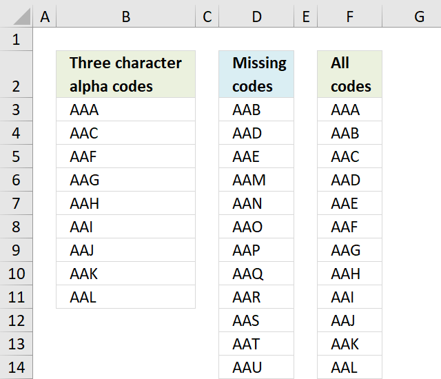
2. Identify missing three character alpha code numbers
This blog article answers a comment in this blog article: Identify missing values in two columns using excel formula
Question: I need to do exactly the same thing, but with three character alpha codes instead of numbers. Can anyone help?
There are 26*26*26 = 17,576 different alpha codes beginning with AAA and ending with ZZZ. Column F contains all 17,576 alpha codes.
The formula in cell D3 compares the values in column B with the values in column F and extracts only those who are missing in column B.
Array formula in cell D3:
Explaining array formula in cell D3
Step 1 - Identify missing values
The COUNTIF function counts values based on a condition or criteria, in this case, it counts values in $F$3:$F$17578 based on $B$3:$B$11.
A 0 (zero) indicates a missing value.
COUNTIF($B$3:$B$11, $F$3:$F$17578)=0
becomes
{0;1;0;1;1;0;0;0;0;0;0;0 ... 0}=0
and returns
{TRUE; FALSE; TRUE; FALSE; FALSE; TRUE; TRUE; TRUE; TRUE; TRUE; TRUE; TRUE}
Step 2 - Replace TRUE with corresponding row number
The IF function returns the corresponding row number if boolean value is TRUE. FALSE returns "" (nothing).
IF(COUNTIF($B$3:$B$11, $F$3:$F$17578)=0, MATCH(ROW($F$3:$F$17578), ROW($F$3:$F$17578)), "")
becomes
IF({TRUE; FALSE; TRUE; FALSE; FALSE; TRUE; TRUE; TRUE; TRUE; TRUE; TRUE; TRUE}, MATCH(ROW($F$3:$F$17578), ROW($F$3:$F$17578)), "")
and returns
{"";2;"";4;5;"";"";"";"";"";"" ... ""}
Step 3 - Extract row number
The SMALL function returns the k-th smallest number in a cell range or array. SMALL(array, k)
SMALL(IF(COUNTIF($B$3:$B$11, $F$3:$F$17578)=0, MATCH(ROW($F$3:$F$17578), ROW($F$3:$F$17578)), ""), ROWS($A$1:A1))
becomes
SMALL({"";2;"";4;5;"";"";"";"";"";"" ... ""}, ROWS($A$1:A1))
The ROWS function returns the number of rows in a cell reference, in this case the cell reference expands as the cell is copied to cells below.
SMALL({"";2;"";4;5;"";"";"";"";"";"" ... ""}, ROWS($A$1:A1))
becomes
SMALL({"";2;"";4;5;"";"";"";"";"";"" ... ""}, 1)
and returns 2.
Step 4 - Return value
The INDEX function returns a value based on a row and column number. The column number is not needed here.
INDEX($F$3:$F$17578, SMALL(IF(COUNTIF($B$3:$B$11, $F$3:$F$17578)=0, MATCH(ROW($F$3:$F$17578), ROW($F$3:$F$17578)), ""), ROWS($A$1:A1)))
becomes
INDEX($F$3:$F$17578, 2)
and returns "AAB" in cell D3.
Get excel *.xlsm file
I made all the alpha codes using a UDF, you don't need the UDF to extract missing alpha codes so you can disable macros for this workbook if you like.
Three character alpha code.xlsm
3. Insert blank rows for missing values
![]()
I have 2 columns named customer (A1) and OR No. (B1).
Under customer are names enumerated below them. opposite the name of customers are OR No. issued to various customers.
OR No. is in broken sequence.
My question is, how will I insert the rows for the corresponding missing OR numbers?
Example:
(A1) (B1)
Customer OR No.
customer 1 1
customer 2 2
customer 3 5
customer 4 7
customer 5 8
customer 6 10
customer 7 11
customer 8 13
customer 9 14
customer 10 15
Answer:
The solution presented below does not insert blank rows for missing values. I am going to create a new list based on the old list, however, it will have blank rows for missing values.
We don't need to use a macro if we do it this way, a simple formula is enough.
Create new OR numbers
- Type 1 in cell B2.
- Select cell B2
- Press and hold with right mouse button on black dot on cell B2.

- Drag down to cell B16.

- Press with left mouse button on "Fill series"
Match OR number and return customer name

Formula in cell A2:
Copy cell A2 and paste to cell range A3:A16.
This formula matches the OR number and returns the Customer. If a customer is not found, the cell becomes blank.
Explaining formula in cell A2
Step 1 - Find position of given value in column
The MATCH function returns the relative position of a specific value in a list. It returns the first position of the first instance found, if duplicates in the list.
MATCH(Sheet2!B2, Sheet1!$B$2:$B$11, 0)
becomes
MATCH(1, {1; 2; 5; 7; 8; 10; 11; 13; 14; 15}, 0)
and returns 1.
Step 2 - Return value based on position
The INDEX function returns a value based ona a row number and a column number if needed.
INDEX(Sheet1!$A$2:$A$11,MATCH(Sheet2!B2, Sheet1!$B$2:$B$11, 0))
becomes
INDEX(Sheet1!$A$2:$A$11,1)
becomes
INDEX({"customer 1"; "customer 2"; "customer 3"; "customer 4"; "customer 5"; "customer 6"; "customer 7"; "customer 8"; "customer 9"; "customer 10"},1)
and returns "customer 1" in cell A2.
Step 3 - Return blank if no value is found
The IFERROR function returns a blank value "" if the formula returns an error, this will return a blank cell if a number is missing.
The IFERROR function catches all kinds of errors in your formula, use with caution.
IFERROR(INDEX(Sheet1!$A$2:$A$11,MATCH(Sheet2!B2, Sheet1!$B$2:$B$11, 0)), "")
4. Identify missing numbers in two columns based on a numerical range

Question:
I want to find missing numbers in two ranges combined? They are not adjacent.
Answer:
Array formula in cell B5:
How to create an array formula
- Select cell B5
- Press with left mouse button on in formula bar
- Copy and paste array formula to formula bar
- Press and hold Ctrl + Shift
- Press Enter
- Release all keys
To remove #NUM errors, Excel 2007 users can use this formula:
Named ranges
List1 (A2:A6)
List2 (E4:E6)
missing_list_start (B5)
What is named ranges?
Explaining array formula in cell B5
=SMALL(IF((COUNTIF(List1, ROW(INDEX($A:$A, $F$2):INDEX($A:$A, $F$3)))+COUNTIF(List2, ROW(INDEX($A:$A, $F$2):INDEX($A:$A, $F$3))))=0, ROW(INDEX($A:$A, $F$2):INDEX($A:$A, $F$3)), ""), ROW(A1)))
Step 1 - Create dynamic array with numbers from start to end
=SMALL(IF((COUNTIF(List1, ROW(INDEX($A:$A, $F$2):INDEX($A:$A, $F$3)))+COUNTIF(List2, ROW(INDEX($A:$A, $F$2):INDEX($A:$A, $F$3))))=0, ROW(INDEX($A:$A, $F$2):INDEX($A:$A, $F$3)), ""), ROW(A1)))
ROW(INDEX($A:$A, $F$2):INDEX($A:$A, $F$3))
becomes
ROW(INDEX($A:$A, 1):INDEX($A:$A, 10))
becomes
ROW($A$1:INDEX($A:$A, 10))
becomes
ROW($A$1:$A$10)
and returns this array:
{1; 2; 3; 4; 5; 6; 7; 8; 9; 10}
Step 2 - Find missing numbers
=SMALL(IF((COUNTIF(List1, ROW(INDEX($A:$A, $F$2):INDEX($A:$A, $F$3)))+COUNTIF(List2, ROW(INDEX($A:$A, $F$2):INDEX($A:$A, $F$3))))=0, ROW(INDEX($A:$A, $F$2):INDEX($A:$A, $F$3)), ""), ROW(A1)))
(COUNTIF(List1, ROW(INDEX($A:$A, $F$2):INDEX($A:$A, $F$3)))+COUNTIF(List2, ROW(INDEX($A:$A, $F$2):INDEX($A:$A, $F$3))))
becomes
(COUNTIF(List1, {1; 2; 3; 4; 5; 6; 7; 8; 9; 10})+COUNTIF(List2, {1; 2; 3; 4; 5; 6; 7; 8; 9; 10}))
becomes
(COUNTIF({1;3;4;7;8}, {1; 2; 3; 4; 5; 6; 7; 8; 9; 10})+COUNTIF({1;2;5}, {1; 2; 3; 4; 5; 6; 7; 8; 9; 10}))
{0;1;1;0;0;1;1;0;0} + {1;0;0;1;0;0;0;0;0}
and returns
{1;1;1;1;0;1;1;0;0}
Step 3 - Convert boolean array into missing numbers
=SMALL(IF((COUNTIF(List1, ROW(INDEX($A:$A, $F$2):INDEX($A:$A, $F$3)))+COUNTIF(List2, ROW(INDEX($A:$A, $F$2):INDEX($A:$A, $F$3))))=0, ROW(INDEX($A:$A, $F$2):INDEX($A:$A, $F$3)), ""), ROW(A1)))
IF((COUNTIF(List1, ROW(INDEX($A:$A, $F$2):INDEX($A:$A, $F$3)))+COUNTIF(List2, ROW(INDEX($A:$A, $F$2):INDEX($A:$A, $F$3))))=0, ROW(INDEX($A:$A, $F$2):INDEX($A:$A, $F$3)), "")
becomes
IF(({1;1;1;1;0;1;1;0;0}, ROW(INDEX($A:$A, $F$2):INDEX($A:$A, $F$3)), "")
becomes
IF(({1;1;1;1;0;1;1;0;0}, {1; 2; 3; 4; 5; 6; 7; 8; 9; 10}, "")
and returns
{"";"";"";"";6;"";"";9;10}
Step 4 - Return the k-th smallest number
=SMALL(IF((COUNTIF(List1, ROW(INDEX($A:$A, $F$2):INDEX($A:$A, $F$3)))+COUNTIF(List2, ROW(INDEX($A:$A, $F$2):INDEX($A:$A, $F$3))))=0, ROW(INDEX($A:$A, $F$2):INDEX($A:$A, $F$3)), ""), ROW(A1)))
becomes
=SMALL({"";"";"";"";6;"";"";9;10}, ROW(A1))
becomes
=SMALL({"";"";"";"";6;"";"";9;10}, 1)
returns the number 6 in cell B5.
How to customize the formula to your excel spreadsheet
Change the named ranges.
Get excel sample file for this tutorial.
missing-values-in-two-columns.xlsx
(Excel 2007 Workbook *.xlsx)
5. Identify missing numbers in two columns combined based on a numerical range - Excel 365

Formula in cell F8:
Explaining formula
FILTER(SEQUENCE(G3-G2+1,,G2),ISERROR(MATCH(SEQUENCE(G3-G2+1,,G2),VSTACK(B3:B7,D3:D5),0)))
Step 1 -
SEQUENCE(G3-G2+1,,G2)
Macro category
Table of Contents How to create an interactive Excel chart How to filter chart data How to build an interactive […]
Table of Contents Excel monthly calendar - VBA Calendar Drop down lists Headers Calculating dates (formula) Conditional formatting Today Dates […]
Table of Contents Split data across multiple sheets - VBA Add values to worksheets based on a condition - VBA […]
Missing values category
More than 1300 Excel formulasExcel categories
30 Responses to “Find missing numbers”
Leave a Reply
How to comment
How to add a formula to your comment
<code>Insert your formula here.</code>
Convert less than and larger than signs
Use html character entities instead of less than and larger than signs.
< becomes < and > becomes >
How to add VBA code to your comment
[vb 1="vbnet" language=","]
Put your VBA code here.
[/vb]
How to add a picture to your comment:
Upload picture to postimage.org or imgur
Paste image link to your comment.
Hi Oscar,
Thanks for the reply and the time to help me on this one.
You are a big help.
God bless you always.
If this operation needs to be done repeatedly, perhaps using a macro would be a more useful alternative...
Sub InsertMissingRows() Dim X As Long, LastRow As Long, Difference As Long Const OrderColumn As String = "B" Const StartRow As Long = 2 LastRow = Cells(Rows.Count, OrderColumn).End(xlUp).Row For X = LastRow To StartRow + 1 Step -1 Difference = Cells(X, OrderColumn).Value - Cells(X - 1, OrderColumn) If Difference > 1 Then Rows(X).Resize(Difference - 1).Insert End If Next LastRow = Cells(Rows.Count, OrderColumn).End(xlUp).Row Cells(StartRow, OrderColumn).Resize(LastRow - StartRow + 1). _ SpecialCells(xlCellTypeBlanks).FormulaR1C1 = "=1+R[-1]C" Columns("B").Value = Columns("B").Value End SubHughMark,
You are welcome!
Rick Rothstein (MVP - Excel),
Thanks for your contribution!
hi,
how can we extend the same to 8000 rows in a column,
creating array formula as you said is not working
Select cell B5
Copy / Paste array formula
Press and hold Ctrl + Shift
Press Enter
Release all keys
what should i do to continue ,
any alternative method to copy the array formula
expecting a reply at the earliest
anchal j vattakunnel,
Adjust cell range (bolded)
=SMALL(IF(ISERROR(MATCH($C$1+ROW(OFFSET($A$1, 0, 0, $C$2-$C$1+1))-1, $A$2:$A$6, 0)), $C$1+ROW(OFFSET($A$1, 0, 0, $C$2-$C$1+1))-1), ROW(A1))
Just wanted to say thanks. This worked on a huge range of data that I had. Really appreciate it!
hi
i have 65000 nos in a column how can in find the missing nos. the above formula cannot work.... please help me to rectify the problem. very urgent...
I couldn't get the formula to work either, by changing the range. Could you please help me also with out using VBA?
Thanks
Kenneth G,
How large is your range?
1-3660
The formula should work. Can you provide your formula? Did you create an array formula?
was not hitting ctrl+shift+enter. it works now!
Dear All,
I have serial numbers from 1 to 40,000 entry in excel. In-between serial numbers there some missing numbers. How can I findout what are the missing numbers from large serial numbers i.e. 1 to 40,000.
For e.g. there are serial numbers 1, 2, 4, 5, 6, 8, 9, 10 like wise i have 60,000numbers. Here missing numbers are 3, 7. How I will findout missing numbers 3 & 7 easily.
Kindly help me.
With advance thanks.
Regards,
Nihar
XLRI
abu and ravi,
I have added a vba solution to this post: Missing numbers (vba)
I want to find missing numbers starting from 80000001 to 80003200, how to find it by VBA code, Excel gets hang after entering VBA code.
Chetan Sonawane,
Yes, you are right. Try the new file Find-missing-values-version2.xlsm. Link above.
I want to split one single coloum of approximately 12000 values into several coloums so that I can take print of such numbers on pages, plz help me on this. how to do it ?
Chetan Sonawane,
Adjust cell range Sheet1!$A$1:$A$151.
Get the Excel *.xlsx file
Rearrange-data-from-a-column-to-multiple-columns.xlsx
Thank you Oscar very much, due to your help my work is getting easy. I tried spliting 12935 values in Excel using MS Office 2007, but the file works very slowly , Shall I install MS Office 2010 ?, will it work more faster ? I want your Advice.
I want to find missing value staring with alphabets like B00001 to B11221, how to find it by VBA code, please post new code.
Dear sir,
I wish to find missing nos. starting with alphabets like S0001 to S1122, Please send the code.
How to find missing nos which starts with B0001 or S-001
Dear Osacar Sir,
Please send me solution for finding missing nos starting with J000001 or S000001
Chetan Sonawane,
Create a new column and remove J and S from your lists.
If your list is in column A, cell B1:
=RIGHT(A1,LEN(A1)-1)*1
Copy formula downwards as far as needed.
Start macro and use it on column B.
Dear Sir,
Instead of formula can you help me with VBA code, If you can please modify VBA code for finding missing nos starting with J000001 or S000001
How i can put values of missing sequential numbers?
Number values
1 30
4 20
missing number 2 having value 10
missing number 3 having value 50
Hi Oscar,
I have tried the Array Formula, however, when i hit CTRL+Shift+Enter nothing happens. All the fields are highlighted but it does not provide any info. Any ideas?
Please help
how to use multi user in single macro program sir
Hi,
Kindly assist in finding the missing number in a specific range with dash along with the numbers.
Sample data.
385-234-4980
Hi sir,
SMALL(IF(ISERROR(MATCH(ROW(INDIRECT($E$2&":"&$E$3)),$B$3:$B$7,0)),ROW(INDIRECT($E$2&":"&$E$3))),ROWS($D$8:D8))
Same concept but with different construction..,,