Sort a column alphabetically
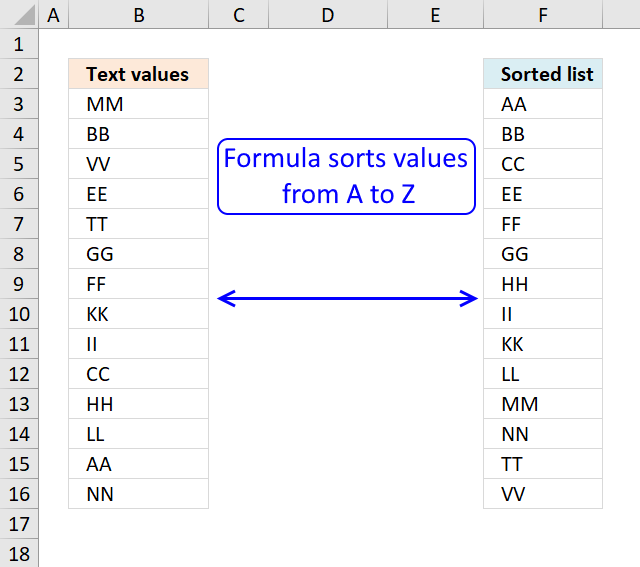
Table of Contents
- Sort a column - Excel 365
- Sort a column using array formula
- Two columns sorting by the second column - Excel 365
- Two columns sorting by the second column
- Sort alphanumeric values
- Sort text values by length
- Sort two columns
- Sort records based on two columns
- Sort items by adjacent number in every other value - Array formula
- Sort items by adjacent number in every other value - Excel 365 formula
- Sort items by adjacent number in every other value vertically
- Reverse a list ignoring blanks
- Reverse a list ignoring blanks - Excel 365
- Reverse a list ignoring blanks - manual steps
- Sort a multi-column cell range from A to Z - array formula for older Excel versions
1. Sort a column - Excel 365

Excel 365 formula in cell D3:
The SORT function sorts values from a cell range or array
Function syntax: SORT(array,[sort_index],[sort_order],[by_col])
2. Sort a column using array formula
I am inspired once again by the article Sorting Text in Excel using Formulas at Pointy haired Dilbert. In Chandoo´s article, he sorts text with a "helper" column. My goal with this article is to show you how to sort text cells alphabetically without a helper column.
Here is an example, cell range $A$2:$A$15 contains text values.
Here is how to automatically sort text cells without any user interaction in cell B2:
Array formula in cell B2:
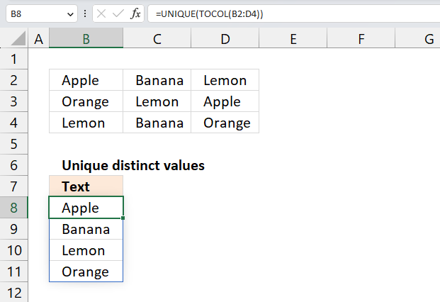
This article demonstrates how to filter a unique distinct list sorted from A to Z:
Extract a unique distinct list sorted from A to Z
The following post shows you how to sort and filter duplicate values alphabetically:
Extract a list of alphabetically sorted duplicates from a column
Learn how to sort a multi-column cell range alphabetically and display the values in a single column:
Sort a range from A to Z [Array formula]
Sort a data set using an array formula:
How to sort a data set using three different approaches, built-in tools, array formulas, and VBA
Tip! You can sort a data set in any way you like it, if you convert it to an excel defined table: Excel table - Sort data
How to create an array formula
- Copy (Ctrl + c) and paste (Ctrl + v) array formula into formula bar.
- Press and hold Ctrl + Shift.
- Press Enter once.
- Release all keys.
Copy cell B2 and paste it down as far as needed.
Explaining array formula in cell B2
Step 1 - Count "smaller" values
COUNTIF(range,criteria) counts the number of cells within a range that meet the given condition
COUNTIF($A$2:$A$15, "<"&$A$2:$A$15)
becomes
COUNTIF({MM,BB,VV,EE,TT,GG,FF,KK,KK,II,CC,HH,LL,AA,NN}, "<"&MM,"<"&BB,"<"&VV,"<"&EE,"<"&TT,"<"&GG,"<"&FF,"<"&KK,"<"&II,"<"&CC,"<"&HH,"<"&LL,"<"&AA,"<"&NN)
The first value in this array formula is "MM". Let´s see what happens when COUNTIF calculates how many values is small than "MM".
COUNTIF({MM,BB,VV,EE,TT,GG,FF,KK,II,CC,HH,LL,AA,NN}, "<"&"MM"
becomes
COUNTIF({MM"<"&"MM",BB"<"&"MM",VV"<"&"MM",EE"<"&"MM",TT"<"&"MM",GG"<"&"MM",FF"<"&"MM",KK"<"&"MM",II"<"&"MM",CC"<"&"MM",HH"<"&"MM",LL"<"&"MM",AA"<"&"MM",NN"<"&"MM"}
MM<MM is FALSE and BB<MM is TRUE and so on.. The array becomes:
COUNTIF({FALSE, TRUE, FALSE, TRUE, FALSE, TRUE, TRUE, TRUE, TRUE, TRUE, TRUE, TRUE, TRUE, FALSE}
becomes
COUNTIF({0, 1, 0, 1,0, 1 , 1 ,1 ,1 ,1 ,1 ,1 ,1 ,1 ,1 ,1 ,0} and the total is 10 which is the first number in the returning array. 0+1+0+1+0+1+1+1+1+1+1+1+1+1+1+1+0 = 10
Next is COUNTIF({MM,BB,VV,EE,TT,GG,FF,KK,II,CC,HH,LL,AA,NN}, "<"&"BB")
becomes
COUNTIF({MM"<"&"BB",BB"<"&"BB",VV"<"&"BB",EE"<"&"BB",TT"<"&"BB",GG"<"&"BB",FF"<"&"BB",KK"<"&"BB",II"<"&"BB",CC"<"&"BB",HH"<"&"BB",LL"<"&"BB",AA"<"&"BB",NN"<"&"BB"})
becomes
COUNTIF({FALSE, FALSE, FALSE, FALSE, FALSE, FALSE, FALSE, FALSE, FALSE, FALSE, FALSE,FALSE , TRUE, FALSE})
becomes
COUNTIF({0, 0, 0, 0,0, 0, 0,0,0,0,0,0,0,0,0,1,0}) and the total is 1 which is the second number in the returning array.
and so on...
COUNTIF($A$2:$A$15, "<"&$A$2:$A$15) returns this array:
{10, 1,13,3,12,5,4,8,7,2,6,9,0,11}
Step 2 - Return the k-th smallest number in array
SMALL(array,k) returns the k-th smallest row number in this data set.
SMALL({10, 1,13,3,12,5,4,8,7,2,6,9,0,11}, ROW(1:1)) returns the smallest number in this data set, 0 (zero).
Step 3 - Find position in array
MATCH(lookup_value;lookup_array; [match_type]) returns the relative position of an item in an array that matches a specified value
MATCH(SMALL(COUNTIF($A$2:$A$15, "<"&$A$2:$A$15), ROW(1:1)), COUNTIF($A$2:$A$15, "<"&$A$2:$A$15), 0)
becomes
MATCH(0, {10, 1,13,3,12,5,4,8,7,2,6,9,0,11}, 0) and returns 13.
Step 4 - Return value
INDEX(array,row_num,[column_num]) returns a value or reference of the cell at the intersection of a particular row and column, in a given range.
=INDEX($A$2:$A$15, MATCH(SMALL(COUNTIF($A$2:$A$15, "<"&$A$2:$A$15), ROW(1:1)), COUNTIF($A$2:$A$15, "<"&$A$2:$A$15), 0))
becomes
INDEX($A$2:$A$15, 13)
and returns AA in cell B2.
Get Excel sample file for this tutorial
Sorting-text-cells-using-array-formulas.xls
(Excel 97-2003 Workbook *.xls)
3. Sort two columns by the second column - Excel 365

Excel 365 is a lot more easy to work with, the new SORTBY function makes everything so simple when it comes to sorting values.
Excel 365 dynamic array formula in cell E3:
The SORTBY function spills values below and to the right of cell E3 as far as needed. A #SPILL error indicates that one or more cells are not empty. Delete the nonempty cell values and the formula works again.
The SORTBY function sorts a cell range or array based on values in a corresponding range or array.
Function syntax: SORTBY(array, by_array1, [sort_order1], [by_array2, sort_order2],…)
4. Sort two columns by the second column

These formulas are for earlier Excel versions than Excel 365, the image above shows a list of dates and corresponding values in cell range A2:B9.
The formulas in cell range D2:D9 and E2:E9 sort the values from small to large based on column B. Note that you can sort numbers just using the SMALL function, however, this formula in cell D2 also sorts text values from A to Z.
Array Formula in cell E2:
Array Formula in cell D2:
Get excel *.xlsx
Two columns sorting by the second column.xlsx
6. Sort text values by length
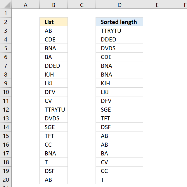
The image above demonstrates a formula in cell D3 that sorts values based on character length, the value with the most characters are at the top, and the value with the least amount of characters is at the bottom.
Excel 365 dynamic array formula in cell D3:
I recommend Excel 365 users read this article: Sort by word length for how the formula works step by step. The following formula is for earlier Excel versions.
Array formula in D3:
copied down as far as needed.
To enter an array formula, type the formula in a cell then press and hold CTRL + SHIFT simultaneously, now press Enter once. Release all keys.
The formula bar now shows the formula with a beginning and ending curly bracket telling you that you entered the formula successfully. Don't enter the curly brackets yourself.
Explaining formula in cell B2
Step 1 - Calculate the k-th largest string length
In order to return a new value in each cell, the formula uses an expanding cell reference to return the next largest value. The LEN function returns the character length of a value, the ROWS function returns the number of rows in a cell reference. The LARGE function returns the k-th largest value. LARGE( array, k)
LARGE(LEN($B$3:$B$20), ROWS($A$1:A1))
becomes
LARGE(LEN($B$3:$B$20), 1)
becomes
LARGE({2; 3; 3; 2; 4; 3; 3; 3; 2; 6; 4; 3; 3; 2; 3; 1; 3; 2}, 1)
and returns 6.
Step 2 - Check previously displayed values in cells above
The COUNTIF function counts cells in cell range based on a condition or criteria. The first argument contains an expanding cell reference that lets the formula keep track of already shown values.
COUNTIF($F$2:F2, $B$3:$B$20)
becomes
COUNTIF("Sorted length",{"AB"; "CDE"; "BNA"; "BA"; "DDED"; "KJH"; "LKJ"; "DFV"; "CV"; "TTRYTU"; "DVDS"; "SGE"; "TFT"; "CC"; "BNA"; "T"; "DSF"; "AB"})
and returns
{0;0;0;0;0;0;0;0;0;0;0;0;0;0;0;0;0;0}
Step 3 - Check if the count of prior values are less than the total count of each value
(COUNTIF($D$2:D2,$B$3:$B$20)<COUNTIF($B$3:$B$20,$B$3:$B$20)
becomes
{0; 0; 0; 0; 0; 0; 0; 0; 0; 0; 0; 0; 0; 0; 0; 0; 0; 0}<{2; 1; 2; 1; 1; 1; 1; 1; 1; 1; 1; 1; 1; 1; 2; 1; 1; 2}
and returns
{TRUE; TRUE; TRUE; TRUE; TRUE; TRUE; TRUE; TRUE; TRUE; TRUE; TRUE; TRUE; TRUE; TRUE; TRUE; TRUE; TRUE; TRUE}.
Step 4 - Match length to array
The MATCH function returns the relative position in a cell range or array of a given value.
MATCH(LARGE(LEN($B$3:$B$20), ROWS($A$1:A1)), LEN($B$3:$B$20)*(COUNTIF($F$2:F2, $B$3:$B$20)<COUNTIF($B$3:$B$20, $B$3:$B$20)), 0)
becomes
MATCH(6, LEN($B$3:$B$20)*(COUNTIF($F$2:F2, $B$3:$B$20)<COUNTIF($B$3:$B$20, $B$3:$B$20)), 0)
becomes
MATCH(6, LEN($B$3:$B$20)*{TRUE; TRUE; TRUE; TRUE; TRUE; TRUE; TRUE; TRUE; TRUE; TRUE; TRUE; TRUE; TRUE; TRUE; TRUE; TRUE; TRUE; TRUE}, 0)
becomes
MATCH(6, {2; 3; 3; 2; 4; 3; 3; 3; 2; 6; 4; 3; 3; 2; 3; 1; 3; 2}*{TRUE; TRUE; TRUE; TRUE; TRUE; TRUE; TRUE; TRUE; TRUE; TRUE; TRUE; TRUE; TRUE; TRUE; TRUE; TRUE; TRUE; TRUE}, 0)
becomes
MATCH(6, {2; 3; 3; 2; 4; 3; 3; 3; 2; 6; 4; 3; 3; 2; 3; 1; 3; 2}, 0)
and returns 10.
Step 5 - Return value
The INDEX function returns a value based on row number (and column number if needed)
INDEX($B$3:$B$20, MATCH(LARGE(LEN($B$3:$B$20), ROWS($A$1:A1)), LEN($B$3:$B$20)*(COUNTIF($F$2:F2, $B$3:$B$20)<COUNTIF($B$3:$B$20, $B$3:$B$20)), 0))
becomes
INDEX($B$3:$B$20, 10)
amd returns TTRYTU in cell D3.
Get Excel *.xlsx file
Sort text based on lengthv2.xlsx
7. Sort two columns
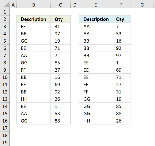
The image above shows a table with two columns in cell range B3:C16, it contains random text values in column B and random numbers in column C. The array formula in cell E3 sorts the text values in column B from A to Z, the array formula in cell F3 sorts the numbers in column C based on the adjacent value in column E.
In other words, the records are sorted based on the text value and then on numbers.
Array formula in E3:
To enter an array formula, type the formula in a cell then press and hold CTRL + SHIFT simultaneously, now press Enter once. Release all keys.
The formula bar now shows the formula with a beginning and ending curly bracket telling you that you entered the formula successfully. Don't enter the curly brackets yourself.
Array formula in F3:
Explaining formula in cell E3
Step 1 - Create an array of numbers representing the rank order if the list were sorted
The COUNTIF function counts values based on a condition or criteria, in this case, we use the < less than sign to compare the value against all other values.
COUNTIF($B$3:$B$16, "<"&$B$3:$B$16)
becomes
COUNTIF({"FF"; "BB"; "GG"; "EE"; "AA"; "GG"; "FF"; "BB"; "EE"; "BB"; "HH"; "EE"; "AA"; "GG"},{"<FF"; "<BB"; "<GG"; "<EE"; "<AA"; "<GG"; "<FF"; "<BB"; "<EE"; "<BB"; "<HH"; "<EE"; "<AA"; "<GG"})
and returns
{8; 2; 10; 5; 0; 10; 8; 2; 5; 2; 13; 5; 0; 10}.
Step 2 - Get the k-th smallest number from array
To be able to return a new value in a cell each I use the SMALL function to filter column numbers from smallest to largest.
The ROWS function keeps track of the numbers based on an expanding cell reference. It will expand as the formula is copied to the cells below.
SMALL(COUNTIF($B$3:$B$16, "<"&$B$3:$B$16), ROWS($A$1:A1))
becomes
SMALL({8; 2; 10; 5; 0; 10; 8; 2; 5; 2; 13; 5; 0; 10}, ROWS($A$1:A1))
becomes
SMALL({8; 2; 10; 5; 0; 10; 8; 2; 5; 2; 13; 5; 0; 10}, 1)
and returns 0 (zero).
Step 3 - Find position of number in array
The MATCH function finds the relative position of a value in an array or cell range.
MATCH(SMALL(COUNTIF($B$3:$B$16, "<"&$B$3:$B$16), ROWS($A$1:A1)), COUNTIF($B$3:$B$16, "<"&$B$3:$B$16), 0)
becomes
MATCH(0, COUNTIF($B$3:$B$16, "<"&$B$3:$B$16), 0)
becomes
MATCH(0, {8; 2; 10; 5; 0; 10; 8; 2; 5; 2; 13; 5; 0; 10}, 0)
and returns 5.
Step 4 - Get value
The INDEX function returns a value based on row number (and column number if needed)
INDEX($B$3:$B$16, MATCH(SMALL(COUNTIF($B$3:$B$16, "<"&$B$3:$B$16), ROWS($A$1:A1)), COUNTIF($B$3:$B$16, "<"&$B$3:$B$16), 0))
becomes
INDEX($B$3:$B$16, 5)
and returns "AA" in cell E3.
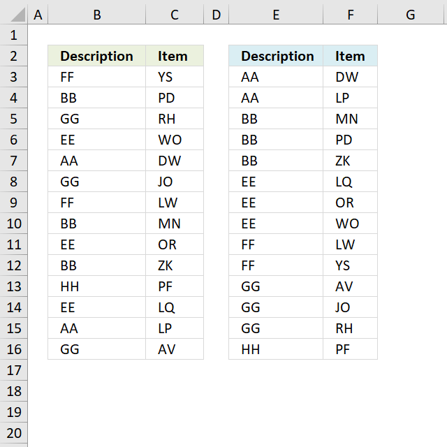
The image above demonstrates a table containing text values in both columns, you need a different array formula to sort the second column now containing text values.
Array formula in E3:
copied down as far as needed.
Array formula in F3:
Get Excel *.xlsx file
Sort two columns using an array formula.xlsx
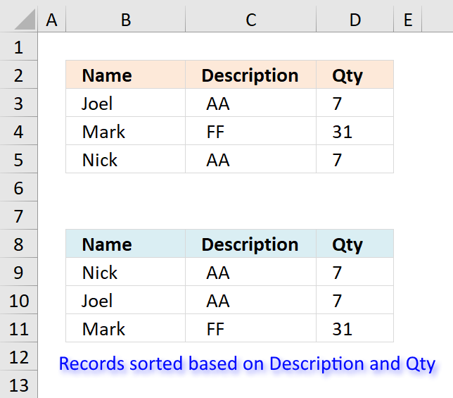
8. Sort records based on two columns
Ralee asks:
If there is information in adjacent columns, say:
Joel, AA, 7
Mark, FF, 31
Nick, AA, 7
with the possibility of matching sort criteria (columns 2 & 3), how would I display the corresponding data after the sort (sorting only columns 2 & 3) without repeats; that is,
Joel, AA, 7
Nick, AA, 7
Mark, FF, 31
Instead of:
Joel, AA, 7
Joel, AA, 7
Mark, FF, 31
?
Answer:
Excel 365 formula in cell B9:
Array formula in B9:
To enter an array formula, type the formula in a cell then press and hold CTRL + SHIFT simultaneously, now press Enter once. Release all keys.
The formula bar now shows the formula with a beginning and ending curly bracket telling you that you entered the formula successfully. Don't enter the curly brackets yourself.
Array formula in C9:
Array formula in D9:
Explaining array formula in cell B9
Step 1 - Create array containing numbers representing rank order if sorted
The COUNTIF function lets you count values based on a condition. The less than sign lets you compare values based on sort order.
COUNTIF($C$3:$C$5, "<"&$C$3:$C$5)
becomes
COUNTIF({" AA";" FF";" AA"},{"< AA";"< FF";"< AA"})
and returns
{0;2;0}
Step 2 - Create rank order based on second column
Integers represent the sort order of column C and decimal values represent the sort order of column D, combining them creates an array that lets you identify the sort order based on both columns.
1/(COUNTIF($D$3:$D$5, ">"&$D$3:$D$5)+1+ROW($D$3:$D$5)/65536)
becomes
1/({0;2;0}+1+ROW($D$3:$D$5)/65536)
becomes
1/({0;2;0}+1+{3;4;5}/65536)
becomes
1/({0;2;0}+1+{0.0000457763671875;0.00006103515625;0.0000762939453125})
becomes
1/({1.00004577636718;3.00006103515625;1.00007629394531})
and returns
{0.9999542257282;0.333326551787276;0.999923711875012}
Step 3 - Add arrays
COUNTIF($C$3:$C$5,"<"&$C$3:$C$5)+(1/(COUNTIF($D$3:$D$5,">"&$D$3:$D$5)+1+ROW($D$3:$D$5)/65536))
becomes
{0;2;0} + {0.9999542257282;0.333326551787276;0.999923711875012}
and returns
{0.9999542257282;2.33332655178728;0.999923711875012}
Step 4 - Extract k-th smallest value in array
To be able to return a new value in a cell each I use the SMALL function to filter column numbers from smallest to largest.
The ROWS function keeps track of the numbers based on an expanding cell reference. It will expand as the formula is copied to the cells below.
SMALL(COUNTIF($C$3:$C$5,"<"&$C$3:$C$5)+(1/(COUNTIF($D$3:$D$5,">"&$D$3:$D$5)+1+ROW($D$3:$D$5)/65536)),ROWS($A$1:A1))
becomes
SMALL({0.9999542257282;2.33332655178728;0.999923711875012},ROWS($A$1:A1))
becomes
SMALL({0.9999542257282;2.33332655178728;0.999923711875012},1)
and returns
0.999923711875012.
Step 5 - Find position of value in array
The MATCH function finds the relative position in a cell range or array.
MATCH(SMALL(COUNTIF($C$3:$C$5,"<"&$C$3:$C$5)+(1/(COUNTIF($D$3:$D$5,">"&$D$3:$D$5)+1+ROW($D$3:$D$5)/65536)),ROWS($A$1:A1)),COUNTIF($C$3:$C$5,"<"&$C$3:$C$5)+(1/(COUNTIF($D$3:$D$5,">"&$D$3:$D$5)+1+ROW($D$3:$D$5)/65536)),0)
becomes
MATCH(0.999923711875012,COUNTIF($C$3:$C$5,"<"&$C$3:$C$5)+(1/(COUNTIF($D$3:$D$5,">"&$D$3:$D$5)+1+ROW($D$3:$D$5)/65536)),0)
becomes
MATCH(0.999923711875012, {0.9999542257282;2.33332655178728;0.999923711875012},0)
and retrurns 3.
Step 6 - Return corresponding value based on position
The INDEX function returns a value based on a cell reference and column/row numbers.
INDEX($B$3:$B$5,MATCH(SMALL(COUNTIF($C$3:$C$5,"<"&$C$3:$C$5)+(1/(COUNTIF($D$3:$D$5,">"&$D$3:$D$5)+1+ROW($D$3:$D$5)/65536)),ROWS($A$1:A1)),COUNTIF($C$3:$C$5,"<"&$C$3:$C$5)+(1/(COUNTIF($D$3:$D$5,">"&$D$3:$D$5)+1+ROW($D$3:$D$5)/65536)),0))
becomes
INDEX($B$3:$B$5,3)
and returns "Nick in cell B9.
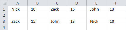
9. Sort items by adjacent number in every other value - Array formula

This section demonstrates formulas that sorts items arranged horizontally based on the adjacent numbers, every other column contains a number.
The image above shows the data in cell range B2:G2 and the array formula in cell B4 sorts the items based on the adjacent number from large to small.
Having data arranged like the image above shows is not something I recommend, it is far better to have the items in one column and the corresponding numbers in the next column.
You can then sort data much easier using the built-in Filter tool or convert the data to an Excel Table which gives you a lot of extra features like formatting and so on.
This article was created to answer the following question.
I have the following situation:
A1, B1, C1, D1, E1, F1
where
A1 = nick
b1 = 10
c1 = zack
d1 = 15
e1 - john
f1 = 13
what formula should i use to get them ordered counting the numbers but names still being associated, like this:
a1 = zack
b1 = 15
c1 = john
d1 = 13
e1 = nick
f1 = 10
Array formula in cell B4:
9.1 How to enter an array formula
- Type the above formula in cell B4.
- Press and hold CTRL + SHIFT keys simultaneously.
- Press Enter once.
- Release all keys.
Copy cell B4 and paste to cells to the right as far as needed.
9.2 Explaining formula in cell B4
Step 1 - Calculate column number
The COLUMN function returns the column number of the top-left cell of a cell reference.
COLUMN(reference)
COLUMN(A1)*0.5
becomes
1*0.5
The asterisk character is a mathematical operator, it multiplies two numbers.
1*0.5 equals 0.5.
Step 2 - Round number to nearest integer
The ROUND function rounds a number based on the number of digits you specify.
ROUND(number, num_digits)
ROUND(COLUMN(A1)*0.5,0)
becomes
ROUNDD(0.5)
and returns 1.
Step 3 - Extract k-th largest number
The LARGE function calculates the k-th largest value from an array of numbers.
LARGE(array, k)
LARGE($B$2:$G$2, ROUND(COLUMN(A1)*0.5, 0))
becomes
LARGE($B$2:$G$2, 1)
becomes
LARGE({"Nick", 10, "Zack", 15, "John", 13}, 1)
and returns 15. 15 is the largest number in the array.
Step 4 - Find relative position
The MATCH function returns the relative position of an item in an array or cell reference.
MATCH(lookup_value, lookup_array, [match_type])
MATCH(LARGE($B$2:$G$2,ROUND(COLUMN(A1)*0.5,0)),$B$2:$G$2,0)
becomes
MATCH(15, $B$2:$G$2,0)
becomes
MATCH(15, {"Nick", 10, "Zack", 15, "John", 13},0)
and returns 4. 15 is the fourth value in the array.
Step 5 - Calculate a number sequence that alternates between 0 (zero) and 1.
The MOD function returns the remainder after a number is divided by a divisor.
MOD(number, divisor)
MOD(COLUMN(A1),2)
becomes
MOD(1,2)
and returns 1.
Step 6 - Calculate position
MATCH(LARGE($B$2:$G$2,ROUND(COLUMN(A1)*0.5,0)),$B$2:$G$2,0)-MOD(COLUMN(A1))
becomes
4-MOD(COLUMN(A1))
becomes
4-1
and returns 3.
Step 7 - Get value
The INDEX function returns a value from a cell range based on a row and column number.
INDEX(array, [row_num], [column_num])
INDEX($B$2:$G$2,MATCH(LARGE($B$2:$G$2,ROUND(COLUMN(A1)*0.5,0)),$B$2:$G$2,0)-MOD(COLUMN(A1),2))
becomes
INDEX($B$2:$G$2,3)
becomes
INDEX({"Nick", 10, "Zack", 15, "John", 13},3)
and returns "Zack" in cell B4.
10. Sort items by adjacent number in every other value - Excel 365 formula

The image above demonstrates a dynamic array formula in cell B4 that sorts and rearranges values based on a horizontal cell range.
Excel 365 formula in cell B4:
The formula above is entered as a regular formula and it works only in Excel 365.
11. Sort items by adjacent number in every other value vertically
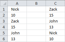
This formula returns data vertically:
12. Reverse a list ignoring blanks

The image above demonstrates a formula in cell D3 that rearranges values, bottom value is now on top etc. It doesn't sort the values at all, however, the example image above has sorted source values in column B and then reverses the values in column D. Sorry for the confusion. The formula in cell C2 is for earlier Excel versions than Excel 365. You will find the Excel 365 in the next section below.
Formula in C2:
To enter an array formula, type the formula in a cell then press and hold CTRL + SHIFT simultaneously, now press Enter once. Release all keys.
The formula bar now shows the formula with a beginning and ending curly bracket telling you that you entered the formula successfully. Don't enter the curly brackets yourself.
Explaining formula in cell D3
Step 1 - Find non-empty cells
$B$3:$B$14<>""
becomes
{"AA"; ""; "BB"; "CC"; ""; "BB"; "DD"; ""; "FF"; "GG"; ""; "HH"}<>""
and returns
{TRUE; FALSE; TRUE; TRUE; FALSE; TRUE; TRUE; FALSE; TRUE; TRUE; FALSE; TRUE}
Step 2 - Replace TRUE with corresponding row value
The IF function returns the row number if cell is not blank. FALSE returns "" (nothing).
IF($B$3:$B$14<>"", MATCH(ROW($B$3:$B$14), ROW($B$3:$B$14)), "")
becomes
IF({TRUE; FALSE; TRUE; TRUE; FALSE; TRUE; TRUE; FALSE; TRUE; TRUE; FALSE; TRUE}, MATCH(ROW($B$3:$B$14), ROW($B$3:$B$14)), "")
becomes
IF({TRUE; FALSE; TRUE; TRUE; FALSE; TRUE; TRUE; FALSE; TRUE; TRUE; FALSE; TRUE}, {1;2;3;4;5;6;7;8;9;10;11;12}, "")
and returns
{1;"";3;4;"";6;7;"";9;10;"";12}
Step 3 - Find k-th largest row number
The LARGE function extracts the k-th smallest number from cell range or array. LARGE(array. k) The second argument contains ROWS($D$1:D1), it has an expanding cell reference that grows when cell is copied to cells below.
LARGE(IF($B$3:$B$14<>"", MATCH(ROW($B$3:$B$14), ROW($B$3:$B$14)), ""), ROWS($D$1:D1))
becomes
LARGE({1;"";3;4;"";6;7;"";9;10;"";12}, ROWS($D$1:D1))
becomes
LARGE({1;"";3;4;"";6;7;"";9;10;"";12}, 1)
and returns 12.
Step 4 - Return value
The INDEX function returns a value based on a row and column number. In this formula the cell range is only in one column, the row number is only needed.
INDEX($B$3:$B$14, LARGE(IF($B$3:$B$14<>"", MATCH(ROW($B$3:$B$14), ROW($B$3:$B$14)), ""), ROWS($D$1:D1)))
becomes
INDEX($B$3:$B$14, 12)
and returns "HH" in cell D3.
Get Excel *.xlsx file
Invert a list ignoring blanks.xlsx
13. Reverse a list ignoring blanks - Excel 365

This example shows an Excel 365 formula that extracts values in cell range B3:B14, ignores blank cells and returns the values starting from the bottom.
Excel 365 dynamic array formula in cell D3:
11.1 Explaining formula
Step 1 - Logical expression
The less than and larger than characters combined lets you filter non-empty values, the result is a boolean value TRUE or FALSE.
B3:B14<>""
becomes
{"AA"; ""; "BB"; "CC"; ""; "BB"; "DD"; ""; "FF"; "GG"; ""; "HH"}<>""
and returns
{TRUE; FALSE; TRUE; TRUE; FALSE; TRUE; TRUE; FALSE; TRUE; TRUE; FALSE; TRUE}.
Step 2 - Filter list excluding blanks
The FILTER function lets you extract values/rows based on a condition or criteria.
FILTER(array, include, [if_empty])
FILTER(B3:B14, B3:B14<>"")
becomes
FILTER({"AA"; ""; "BB"; "CC"; ""; "BB"; "DD"; ""; "FF"; "GG"; ""; "HH"}, {TRUE; FALSE; TRUE; TRUE; FALSE; TRUE; TRUE; FALSE; TRUE; TRUE; FALSE; TRUE})
and returns
{"AA"; "BB"; "CC"; "BB"; "DD"; "FF"; "GG"; "HH"}.
Step 3 - Calculate the number of values in the array
The ROWS function returns the number of rows a given reference or array contains.
ROWS(ref)
ROWS(FILTER(B3:B14,B3:B14<>""))
becomes
ROWS({"AA"; "BB"; "CC"; "BB"; "DD"; "FF"; "GG"; "HH"})
and returns 8.
Step 4 - Create a sequential list of numbers from n to 1
The SEQUENCE function creates a list of sequential numbers.
SEQUENCE(rows, [columns], [start], [step])
SEQUENCE(ROWS(FILTER(B3:B14, B3:B14<>"")), , ROWS(FILTER(B3:B14, B3:B14<>"")), -1)
becomes
SEQUENCE(8, , 8, -1)
and returns {8; 7; 6; 5; 4; 3; 2; 1}.
Step 5 - Get values backwards
The INDEX function returns a value from a cell range, you specify which value based on a row and column number.
INDEX(array, [row_num], [column_num], [area_num])
INDEX(FILTER(B3:B14,B3:B14<>""),SEQUENCE(ROWS(FILTER(B3:B14,B3:B14<>"")),,ROWS(FILTER(B3:B14,B3:B14<>"")),-1))
becomes
INDEX({"AA"; "BB"; "CC"; "BB"; "DD"; "FF"; "GG"; "HH"}, {8; 7; 6; 5; 4; 3; 2; 1})
and returns
{"HH"; "GG"; "FF"; "DD"; "BB"; "CC"; "BB"; "AA"}.
Step 6 - Optimize formula
The LET function lets you name intermediate calculation results which can shorten formulas considerably and improve performance.
LET(name1, name_value1, calculation_or_name2, [name_value2, calculation_or_name3...])
INDEX(FILTER(B3:B14,B3:B14<>""),SEQUENCE(ROWS(FILTER(B3:B14,B3:B14<>"")),,ROWS(FILTER(B3:B14,B3:B14<>"")),-1))
FILTER(B3:B14, B3:B14<>"") is repeated three times in the formula.
x - FILTER(B3:B14, B3:B14<>"")
ROWS(FILTER(B3:B14, B3:B14<>"")) is repeated two times in the formula.
y - ROWS(x)
LET(x, FILTER(B3:B14, B3:B14<>""), y, ROWS(x), INDEX(x, SEQUENCE(y, , y, -1)))
14. Reverse a list ignoring blanks - manual steps

Create a list of numbers next to the list or table.
- Type 1 in the first cell.
- Type 2 in the next cell below.
- Select both cells.
- Press and hold with left mouse button on the dot in the lower right corner of the selection.
- Drag with mouse as far as needed.
- Release left mouse button.

- Select all cells, see the image above.
- Press CTRL + SHIFT + L to apply the Excel FILTER feature. Filter buttons appear at the top cells.

- Press with left mouse button on the right button, a popup menu appears.
- Press with mouse on "Sort Largest to Smallest".

- Press with left mouse button on the left button, and a popup menu appears.

- Press with left mouse button on the check box next to blanks to deselect it, see the image above.
- Press with left mouse button on the OK button.

Press CTRL + SHIFT + L to disable the Excel Filter. Delete the numbers next to the list.
15. Sort a multi-column cell range from A to Z - array formula for older Excel versions
Question: How do I sort a range alphabetically using excel array formula?
Answer:
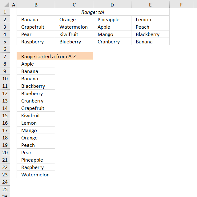
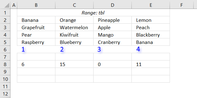
Cell range $B$2:$E$5 contains text values in random order, the formula in cell B8 extracts values sorted from A to Z.
Array formula in B8:
Filter unique distinct values sorted from A to Z with no blanks from a multi-column and multi-row cell range:
Recommended articles
This article demonstrates formulas that extract sorted unique distinct values from a cell range containing also blanks. Unique distinct values […]
How to enter an array formula
- Double press with left mouse button on cell B8
- Copy an paste above formula
- Press and hold CTRL + SHIFT simultaneously
- Press Enter once
Learn how to filter unique distinct values from a multi-column and multi-row cell range:
Recommended articles
This article demonstrates ways to list unique distinct values in a cell range with multiple columns. The data is not […]
How to implement array formula to your workbook
If your list starts at, for example, F2. Change $B$8:B8 in the above formula to F2:$F$2.
The following article demonstrates how to filter a unique distinct list sorted from A to Z, from a multi-column and multi-row cell range:
Recommended articles
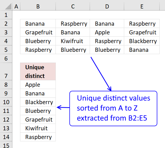
The image above shows an array formula in cell B8 that extracts unique distinct values sorted alphabetically from cell range […]
How to copy array formula
Copy cell B8 and paste to cells below.
How to filter duplicate values from a multi-column and multi-row cell range:
Recommended articles
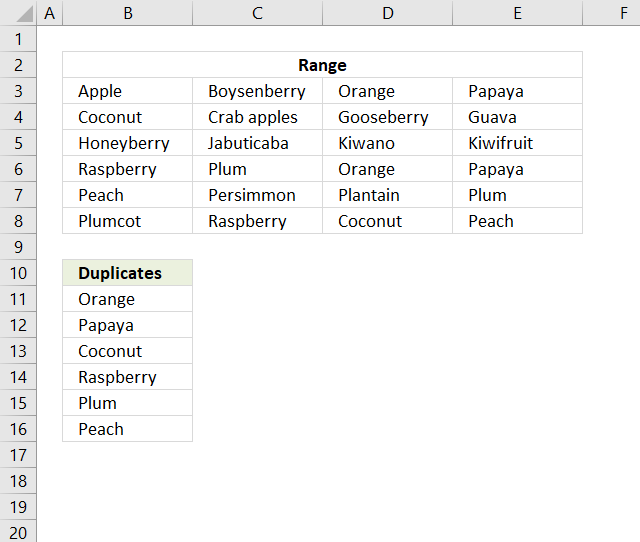
This article describes two formulas that extract duplicates from a multi-column cell range, the first one is built for Excel […]
Explaining formula in cell B8
Step 1 - Rank values based on their relative position if they were sorted
The COUNTIF function counts cells based on a condition, however, in this case, I am using a cell range instead of a single cell in the second argument.
Also, the ampersand & concatenates each value with a less than sign. This makes the COUNTIF function compare each value against the others, the number returned represents the corresponding values position if the list were sorted.
COUNTIF($B$2:$E$5,"<"&$B$2:$E$5)
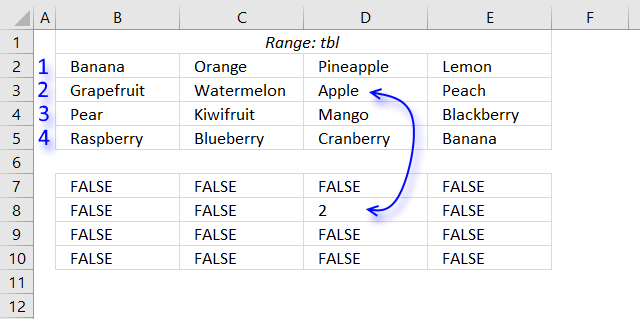
returns {1, 10, 13, 8; 6, 15, 0, 11; 12, 7, 9, 3; 14, 4, 5, 1}.
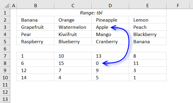
The image above shows the array in cell range B7:E10, "Apple" is 0 (zero) which is the first position if the list were sorted.
Step 2 - Extract the k-th smallest value in array
The SMALL function lets you get the k-th smallest value from a cell range or array.
SMALL(array, k)
SMALL(COUNTIF($B$2:$E$5, "<"&$B$2:$E$5), ROWS($B$8:B8))
The ROWS function allows you to keep track of the number of cells, the cell reference is expanding as we copy the formula and paste to cells below.
SMALL({1, 10, 13, 8; 6, 15, 0, 11; 12, 7, 9, 3; 14, 4, 5, 1}, ROWS($B$8:B8))
becomes
SMALL({1, 10, 13, 8; 6, 15, 0, 11; 12, 7, 9, 3; 14, 4, 5, 1}, 1) and returns 0 (zero).
Step 3 - Compare value to array
The logical expression in the following IF function determines if the value of the position corresponding to the k-th smallest value will be a row number or FALSE.
IF(SMALL(COUNTIF($B$2:$E$5, "<"&$B$2:$E$5), ROWS($B$8:B8))=COUNTIF($B$2:$E$5, "<"&$B$2:$E$5), ROW($B$2:$E$5)-MIN(ROW($B$2:$E$5))+1)
becomes
IF(0=COUNTIF($B$2:$E$5, "<"&$B$2:$E$5), ROW($B$2:$E$5)-MIN(ROW($B$2:$E$5))+1)
becomes
IF(0={1, 10, 13, 8; 6, 15, 0, 11; 12, 7, 9, 3; 14, 4, 5, 1}, ROW($B$2:$E$5)-MIN(ROW($B$2:$E$5))+1)
becomes
IF({FALSE, FALSE, FALSE, FALSE;FALSE, FALSE, TRUE, FALSE;FALSE, FALSE, FALSE, FALSE;FALSE, FALSE, FALSE, FALSE}, ROW($B$2:$E$5)-MIN(ROW($B$2:$E$5))+1)
becomes
IF({FALSE, FALSE, FALSE, FALSE;FALSE, FALSE, TRUE, FALSE;FALSE, FALSE, FALSE, FALSE;FALSE, FALSE, FALSE, FALSE}, {1;2;3;4})
and returns {FALSE, FALSE, FALSE, FALSE;FALSE, FALSE, 2, FALSE;FALSE, FALSE, FALSE, FALSE;FALSE, FALSE, FALSE, FALSE}.
Step 4 - Extract the smallest number from array
The MIN function ignores boolean values TRUE and FALSE.
MIN(IF(SMALL(COUNTIF($B$2:$E$5, "<"&$B$2:$E$5), ROWS($B$8:B8))=COUNTIF($B$2:$E$5, "<"&$B$2:$E$5), ROW($B$2:$E$5)-MIN(ROW($B$2:$E$5))+1))
becomes
MIN({FALSE, FALSE, FALSE, FALSE;FALSE, FALSE, 2, FALSE;FALSE, FALSE, FALSE, FALSE;FALSE, FALSE, FALSE, FALSE})
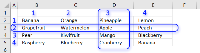
and returns 2. We now know that the first value to be extracted is located on row 2 relative to cell range $B$2:$E$5.
Step 5 - Find column
In this case, the MATCH function returns the relative position horizontally of the value we are looking for.
MATCH(SMALL(COUNTIF($B$2:$E$5,"<"&$B$2:$E$5),ROWS($B$8:B8)),COUNTIF($B$2:$E$5,"<"&INDEX($B$2:$E$5,MIN(IF(SMALL(COUNTIF($B$2:$E$5,"<"&$B$2:$E$5),ROWS($B$8:B8))=COUNTIF($B$2:$E$5,"<"&$B$2:$E$5),ROW($B$2:$E$5)-MIN(ROW($B$2:$E$5))+1)),,1)),0)
becomes
MATCH(SMALL({1, 10, 13, 8; 6, 15, 0, 11; 12, 7, 9, 3; 14, 4, 5, 1},ROWS($B$8:B8)),COUNTIF($B$2:$E$5,"<"&INDEX($B$2:$E$5,MIN(IF(SMALL(COUNTIF($B$2:$E$5,"<"&$B$2:$E$5),ROWS($B$8:B8))=COUNTIF($B$2:$E$5,"<"&$B$2:$E$5),ROW($B$2:$E$5)-MIN(ROW($B$2:$E$5))+1)),,1)),0)
becomes
MATCH(SMALL({1, 10, 13, 8; 6, 15, 0, 11; 12, 7, 9, 3; 14, 4, 5, 1},1),COUNTIF($B$2:$E$5,"<"&INDEX($B$2:$E$5,MIN(IF(SMALL(COUNTIF($B$2:$E$5,"<"&$B$2:$E$5),ROWS($B$8:B8))=COUNTIF($B$2:$E$5,"<"&$B$2:$E$5),ROW($B$2:$E$5)-MIN(ROW($B$2:$E$5))+1)),,1)),0)
becomes
MATCH(0,COUNTIF($B$2:$E$5,"<"&INDEX($B$2:$E$5,MIN(IF(SMALL(COUNTIF($B$2:$E$5,"<"&$B$2:$E$5),ROWS($B$8:B8))=COUNTIF($B$2:$E$5,"<"&$B$2:$E$5),ROW($B$2:$E$5)-MIN(ROW($B$2:$E$5))+1)),,1)),0)
I will be using the INDEX function to extract the values we need based on a row number.
MATCH(0,COUNTIF($B$2:$E$5,"<"&INDEX($B$2:$E$5,MIN(IF(SMALL(COUNTIF($B$2:$E$5,"<"&$B$2:$E$5),ROWS($B$8:B8))=COUNTIF($B$2:$E$5,"<"&$B$2:$E$5),ROW($B$2:$E$5)-MIN(ROW($B$2:$E$5))+1)),,1)),0)
becomes
MATCH(0,COUNTIF($B$2:$E$5,"<"&INDEX($B$2:$E$5,2,,1)),0)
becomes
MATCH(0,COUNTIF($B$2:$E$5,"<"&B3:E3),0)
becomes
MATCH(0,{6,15,0,11},0)
and returns 3. The value we are looking for is in column 3 relative to cell range $B$2:$E$5.
Step 6 - Return value based on row and column
INDEX($B$2:$E$5, MIN(IF(SMALL(COUNTIF($B$2:$E$5, "<"&$B$2:$E$5), ROWS($B$8:B8))=COUNTIF($B$2:$E$5, "<"&$B$2:$E$5), ROW($B$2:$E$5)-MIN(ROW($B$2:$E$5))+1)), MATCH(SMALL(COUNTIF($B$2:$E$5, "<"&$B$2:$E$5), ROWS($B$8:B8)), COUNTIF($B$2:$E$5, "<"&INDEX($B$2:$E$5, MIN(IF(SMALL(COUNTIF($B$2:$E$5, "<"&$B$2:$E$5), ROWS($B$8:B8))=COUNTIF($B$2:$E$5, "<"&$B$2:$E$5), ROW($B$2:$E$5)-MIN(ROW($B$2:$E$5))+1)), , 1)), 0))
becomes
INDEX($B$2:$E$5, 2, 3)
and returns "Apple" in cell B8.
Get Excel *.xlsx file
Sort values category
I will in this article discuss three different techniques to sort a data set in Excel. I am going to […]
Excel categories
102 Responses to “Sort a column alphabetically”
Leave a Reply
How to comment
How to add a formula to your comment
<code>Insert your formula here.</code>
Convert less than and larger than signs
Use html character entities instead of less than and larger than signs.
< becomes < and > becomes >
How to add VBA code to your comment
[vb 1="vbnet" language=","]
Put your VBA code here.
[/vb]
How to add a picture to your comment:
Upload picture to postimage.org or imgur
Paste image link to your comment.
Oscar,
In the part of the formula: 1/(COUNTIF(Qty,">"&Qty)+1))
What is the purpose or logic for divide 1 by the countif (Qty,....)
and
what is the reason for the +1 par of the same formula?
thanks,
Chrisham
chrisham,
Sorry for the late answer.
What is the purpose or logic for divide 1 by the countif (Qty,....)?
The purpose is to sort and find the right "Qty" value for each "Description" value. I know this is a short answer but use "Evaluate Formula" to see each step in formula calculation.
what is the reason for the +1 par of the same formula?
COUNTIF(Qty, ">"&Qty) returns an array containing a zero. 1/0 returns an error. So I had to add 1 to the whole array.
This one did not seem to work. in your excel example file I imputed: a, h,II,b,j,k,c,l,m,d,n,f,p in column A.
The result was
a,a,b,c,d,f,h,II,j,k,l,m,n
but there are not two a's in column a and it seemed to drop p completely... it seems some how shifted... can you help? Thanks.
oops... I did not mean to leave my number for anyone other than you, can you remove it? (how embarrassing)
I figured out the problem I was having. It was simply that if "list" has 15 rows, then both my list content and my output cells NEED to contain 15 items or else funky things happen.
HOWEVER
When I try to do a lengthy list, say of 500 rows, I run into circular reference issues... any thoughts?
Matt,
This one did not seem to work. in your excel example file I imputed: a, h,II,b,j,k,c,l,m,d,n,f,p in column A.
The result was
a,a,b,c,d,f,h,II,j,k,l,m,n
but there are not two a's in column a and it seemed to drop p completely... it seems some how shifted... can you help? Thanks.
The named range contains a blank cell, that is why you get strange results. Change the named range cell reference or replace the named range with a cell reference.
Hi,
I would like to output the unique ID of the sorted list. But when duplicates exist in the original list (in this case ID 1 and 2) it ranks both the BBs as 1.
The formula i have in the Sorted ID List column is =MATCH(SMALL(COUNTIF(List,"<"&List),ROW(1:1)),COUNTIF(List,"<"&List),0)
CURRENT OUTPUT:
ID Text Sorted
values ID list
1 BB 13
2 BB 1
3 VV 1
4 EE 10
5 TT 4
6 GG 7
7 FF 6
8 KK 11
9 II 9
10 CC 8
11 HH 12
12 LL 14
13 AA 5
14 NN 3
Desired Output:
ID Text Sorted
values ID list
1 BB 13
2 BB 1
3 VV 2
4 EE 10
5 TT 4
6 GG 7
7 FF 6
8 KK 11
9 II 9
10 CC 8
11 HH 12
12 LL 14
13 AA 5
14 NN 3
can you please suggest something?
Raj,
=MATCH(SMALL(COUNTIF(List, "<"&List)+ROW(List)/1048576, ROW(1:1)), COUNTIF(List, "<"&List)+ROW(List)/1048576, 0) + CTRL + SHIFT + ENTER. Copy cell and paste it down as far as needed.
adding a countblank statement ensures this working for ranges with blank cells (otherwise the first value will be repeated.
ROW(1:1)+COUNTBLANK(List)
Thanks Oscar, and Thanks Miel for solving my probleme! Cheers and Merry Xmas!
If there is information in adjacent columns, say:
Joel, AA, 7
Mark, FF, 31
Nick, AA, 7
with the possibility of matching sort criteria (columns 2 & 3), how would I display the corresponding data after the sort (sorting only columns 2 & 3) without repeats; that is,
Joel, AA, 7
Nick, AA, 7
Mark, FF, 31
Instead of:
Joel, AA, 7
Joel, AA, 7
Mark, FF, 31
?
Ralee,
read this post: Sort values in parallel in excel, part 2
Great! That's exactly what I needed.
~Thanks
The array formula does not need the SMALL() function to work. You can use this instead : =INDEX(List,MATCH(ROW(List)-MIN(ROW(List)),COUNTIF(List,"<"&List),0)) + cse
Thanks for the COUNTIF() trick.
Jeanbar,
You are right!
Thanks for your contribution!
Oscar,
I found out that the formula you gave to Raj is not working. I think it is due to the "ROW(1:1)" part of it which means nothing. If you want to have a valid rank for the SMALL(Array;rank) you should declare ROW(INDIRECT("1:"&ROWS(List)) as a vector of ranks.
The formula working in my environment is: SORTED LIST =
T(INDEX(LIST,MATCH(SMALL(COUNTIF(LIST,"<"&LIST)+ROW(LIST)/MAX(ROW(LIST)),ROW(INDIRECT("1:"&ROWS(LIST)))),COUNTIF(LIST,"<"&LIST)+ROW(LIST)/MAX(ROW(LIST)),0))) +cse
NB: if one or more entries are blank, they come first in the sorted list.
Jeanbar,
The formula is working here. ROW(1:1) is part of small function which returns k-th smallest value in the dataset. When formula is copied down, Row(1:1) changes to Row(2:2) and then to Row(3:3).
Row(1:1) equals 1
Row(2:2) equals 2
and so on..
Row(1:1) is a relative cell reference.
Maybe you copied the formula into all cells and then presssed CTRL + SHIFT + ENTER?
How to use the formula:
Copy array formula into cell B2 and press Ctrl + Shift + Enter.
Copy CELL B2 and paste it to the cells below, as far as needed.
This is great:)formula worked for me.
But can you explain why we press CTRL + SHIFT + ENTER?
im not an expert.
Jaseel,
I am happy you got the formula working.
The formula is an array formula. To enter the formula as an array formula, type the formula in a cell and then press and hold CTRL + SHIFT and then press ENTER once.
Read more about array formulas: Array formulas
Hi Oscar,
Your formula is great, but I need something greater (I think)
I want to sort multiple columns using formula and even multiple sort types, is it possible?
For Example:
Unsorted Data
==============
Col 1 Col 2
-------------------
B 2
A 1
C 2
A 2
B 1
C 2
Sorted Data must be :
Col 1 Col 2
---------------------
A 1
A 2
B 1
B 2
C 2
C 2
Actually I need the sort type of Col 1 ASC then Col 2 DESC then Col 3 ASC then Col 4 DESC then Col 5 ASC.
But If you could give just the Col 1 ASC then Col 2 ASC formula, it would help me a lot...
Thx
FB,
I think this post answers your question: Sort values in parallel (array formula)
Dear Oscar,
Greatest Help...
Thank you very much
Oscar, can you help me understand the logic behind comparing the array values to themselves? Descr, "<"&Descr
Is there an article I can read somewhere?
Kris,
COUNTIF(Descr, "<"&Descr) compares values in an array and ranks them on their order if they were sorted. COUNTIF({"FF";"BB";"GG";"EE";"AA";"GG";"FF";"BB";"EE";"BB";"HH";"EE";"AA";"GG"}, "<"&{"FF";"BB";"GG";"EE";"AA";"GG";"FF";"BB";"EE";"BB";"HH";"EE";"AA";"GG"}) COUNTIF({"FF"; "BB"; "GG"; "EE"; "AA"; "GG"; "FF"; "BB"; "EE"; "BB"; "HH"; "EE"; "AA"; "GG"}, {; "<"&"BB"; "<"&"GG"; "<"&"EE"; "<"&"AA"; "<"&"GG"; "<"&"FF"; "<"&"BB"; "<"&"EE"; "<"&"BB"; "<"&"HH"; "<"&"EE"; "<"&"AA"; "<"&"GG"}) FF, first value in array becomes: {"FF"&"<"&"FF"; "BB"&"<"&"FF"; "GG"&"<"&"FF"; "EE"&"<"&"FF"; "AA"&"<"&"FF"; "GG"&"<"&"FF"; "FF"&"<"&"FF"; "BB"&"<"&"FF"; "EE"&"<"&"FF"; "BB"&"<"&"FF"; "HH"&"<"&"FF"; "EE"&"<"&"FF"; "AA"&"<"&"FF"; "GG"&"<"&"FF"} becomes {0;1;0;1;1;0;0;1;1;1;0;1;1;0} and the total is 8. COUNTIF(Descr, "<"&Descr) returns {8;2;10;5;0;10;8;2;5;2;13;5;0;10}
there is an error is your named ranges
Qty (B2:B15) should be Qty (d2:d15)
Descr (B2:B15) should be Descr (c2:c15)
Paul,
thanks!
Thanks for formula however if the list has blanks it puts them up top and the data is in the bottom. Since I am using dynamic validation how can i put them up top so the user doesn't have to scroll down for selection?
rivers,
=INDEX(List, MATCH(SMALL(IF(ISBLANK(List), "", COUNTIF(List, "<"&List)), ROW(1:1)), IF(ISBLANK(List), "", COUNTIF(List, "<"&List)), 0))
I'm new to excel array techniques (and loving it), so please forgive me if my question's solution is obvious, but your tip goes a long way toward answering it.
I need to perform an approximate match upon an unsorted table and then lookup an associated value. Because the unsorted table is dynamic and will gain many new rows over time, I need the solution to be formula-based, with no intermediate tables.
Is there a way to build upon this tip to have the sorted arrays in memory? My current strategy would be to use LOOKUP vector function upon the two like-sorted arrays. A MrExcel/ExcelIsFun video demonstrates a related solution (see link below), but the table values are numeric and are sorted directly using SMALL() which won't work upon text data.
Many Thanks!
Mr Excel & excelisfun Trick 36: VLOOKUP w Approximate Match & Unsorted Table
https://www.youtube.com/watch?v=rxhL72gvM5E
Markosys,
That´s a question I don´t have an answer to. It seems overly complicated to create a 2dimensional sorted array when you can use MATCH function to lookup values in an unsorted array.
=INDEX(array, MATCH(lookup_value, array, 0))
Oscar, how would i change your formula if i want to work with COLUMNS rather than ROW... e.g. I have a single row of data in 5 columns, CDAEB and i want formulas in the next 5 columns that results in ABCDE.
I tried swapping the match reference and row(1:1) to column(1:1) but it doesnt work... many thanks.
Themin,
=INDEX($A$1:$A$5, MATCH(SMALL(COUNTIF($A$1:$A$5, "<"&$A$1:$A$5), COLUMN(A:A)), COUNTIF($A$1:$A$5, "<"&$A$1:$A$5), 0)) Get the example file *.xlsx Themin.xlsx
Dear Oscar,
I need array formula if there space empty row in the part of rows 2 until 15, say row 5 and row 10 . so the formula generate exactly the same as your Example.
Please help me on this.
and how can i Sort values Parallel with 4 (four) column or more.
Please tell me why you put "65536" in your array formula
thx
Sergio,
Get the example file:
Sergio.xls
what is the purpose of [COUNTIF(List, "<"&List)]? I tried the same overall formula but I replaced this part with a direct reference to the named range and switched SMALL for LARGE which resulted in the formula below:
=INDEX(List, MATCH(LARGE(List, ROW(1:1)), List, 0))
This produced the same results as your original formula which is what made me wonder why the [COUNTIF(List, "<"&List)] portion needs to be there at all.
Also, in my attempt to understand what this part of the formula is doing I came across something that confused me even more. If the section in question [COUNTIF(List, "<"&List)] is put into cells by itself, without the [INDEX(List...], then the results are dependant on the row where the formula was originally inputted and where the formula was copied. I'm assuming this is because the countif outputs an array but I don't understand why. Can you explain this for me?
I should add that when I said the modified formula produced the same results as the original I meant that both formula's had the SMALL function swapped for the LARGE function.
Hi
I see you are solving a lot of complicated tasks in excel. Though I checked also the link https://www.get-digital-help.com/sorts-values-in-parallel-array-formula/, and many others I can not find the solution for my problem.
I'll explain it a litlle better what i have and what i want to get:
column A ; column B
2 1
2 17
7 11
7 26
3 5
3 19
2 1
2 18
i would like to get first column sorted ascending and second column belonging number to the number of the first column:
column A ; column B
2 1
2 17
2 1
2 18
3 5
3 19
7 11
7 26
I hope you have time to look in to it.
Best regards, Jernej
Jernej,
Is this what you are looking for?
Jernej.xls
in the sort order column i used the array formula you gave to Raj=MATCH(SMALL(COUNTIF(List, "<"&List)+ROW(List)/1048576, ROW(1:1)), COUNTIF(List, "<"&List)+ROW(List)/1048576, 0), and the second column is the text that needs sorting in alphabetical order, in the third column i placed the formula that Chandoo used in his article =VLOOKUP(ROW()-ROW($K$1),$I$2:$J$12,2,FALSE. By doing this helped me to avoid problems with non unique values. I am wondering if u have a way for me to by bass the help column altogether?
Sort Order Info needing Sorting Sorted Info
1 WORK COMPLETE WORK COMPLETE
2 WORK COMPLETE WORK COMPLETE
3 WORK COMPLETE WORK COMPLETE
4 WORK COMPLETE WORK COMPLETE
5 WORK COMPLETE WORK COMPLETE
6 WORK COMPLETE WORK COMPLETE
7 WORK COMPLETE WORK COMPLETE
8 WORK COMPLETE WORK COMPLETE
9 WORK COMPLETE WORK COMPLETE
10 WORK COMPLETE WORK COMPLETE
11 WORK COMPLETE WORK COMPLETE
Hi!
I thank you all for your effort.
I got the right result with the "trick" Anonymous stated in his post. Thanks a lot for answering. This equation will reduce my time behind the screen significantly :).
Best regards, Jernej
Jernej,
Can you give an excel example of the final thing that gave you your desired results.
You wanted above "i would like to get first column sorted ascending and second column belonging number to the number of the first column:
column A ; column B
2 1
2 17
2 1
2 18
3 5
3 19
7 11
7 26"
I need to do the same thing. Sort the first column and then after the sorting is done, put the associated 2nd column next to the first, as you mentioned. I have been successful in sorting the first column.
please help
thanks
could you give me formula for sorting the text with spacing row, and I need next column sorting by first column :
col1 col2
anne 2
marie 3
spacing (text)
jolie 2
linda 5
anne 5
i need name of "anne" converge consecutive in next column like this :
anne 2
anne 5
jolie 2 and so on
please help
thanks
pls can u help how to edit this formula
hi sir pls help how edit this shorting formula. when me was pasting this formula in differnt sheet it show #NA. how i need to apply in my sheet pls expl
great one i love it.one small one i required has u had given a xls to sergio in that if there is an empty in any one error is generated like #NUM!. but me want empty space instead of #NUM!. pls help pls
pardhu,
Create a named range (List) using your cell reference.
Then apply my formula.
pardhu,
Excel 2007:
=IFERROR(INDEX(Descr, MATCH(SMALL(IF(Descr="", "", COUNTIF(Descr, "<"&Descr)), ROW(1:1)), IF(Descr="", "", COUNTIF(Descr, "<"&Descr)), 0)), "") Excel 2003: =IF(ISERROR(INDEX(Descr, MATCH(SMALL(IF(Descr="", "", COUNTIF(Descr, "<"&Descr)), ROW(1:1)), IF(Descr="", "", COUNTIF(Descr, "<"&Descr)), 0))), "", INDEX(Descr, MATCH(SMALL(IF(Descr="", "", COUNTIF(Descr, "<"&Descr)), ROW(1:1)), IF(Descr="", "", COUNTIF(Descr, "<"&Descr)), 0)))
THANK YOU SO MUCH SIR .......... YOUR GREAT
Hi,
I have this data:
12-04-12 1
19-04-12 3
23-04-12 2
01-05-12 1
07-05-12 1
15-05-12 1
05-06-12 1
27-08-12 1
How to get the two column output sorted on the second column using array formula?
Best Regards
Kamal,
See this section: Two columns sorting by the second column
Hello,
I love the formula!
I'm having issues with some of my data being numbers stored as text.
This is the data I have:
AK2
CB4D
23
207
H1
Returned sort:
23
23
AK2
CB4D
H1
Any idea how to solve that?
Cheers,
Ryan,
See attached *.xlsx file
ryan.xlsx
i am very new ing advanced excel. i want to sort from largest to small, but i can't. i need your guidence. Thanx.
Uygar,
Sort from smallest to largest number
Formula
=SMALL($A$2:$A$11, ROW(A1))
Sort from smallest to largest text length
Array formula
=INDEX($A$2:$A$9, MATCH(SMALL(LEN($A$2:$A$9), ROW(A1)), IF(COUNTIF($C$1:C1, $A$2:$A$9)=COUNTIF($A$2:$A$9, $A$2:$A$9), "", LEN($A$2:$A$9)), 0))
How to create an array formula
1. Select cell C2
2. Paste formula
3. Press and hold Ctrl + Shift
4. Press Enter
Get the Excel *.xlsx file
Sort-from-smallest-to-largest.xlsx
Sort 1 Sort 2
1350 1350
1351 1351
1352 1352
1353 1353
1354 1354
1355 1355
9999 1357
1357 1357
1358 1358
1359 1359
1360 1360
1361 1361
1362 1362
1363 1363
1364 1364
9999 9999
9999 9999
9999 9999
9999 9999
9999 9999
9999 9999
9999 9999
I am trying to sort the first column into the second. Wherever the number is 9999 it duplicates what would be the next number. It should be shifting up and moving the 9999 to the end. I am working with data sets of about 200 numbers.
Thanks!
Mark,
Copy cell D1. Paste to cell range D2:D22.
hi, i have a text file and wanted to sort the text file info into different location of row and column in excel.
may i know how can i do that?
inside the text file example:-
header
a1
123
456
a2
123
456
a3
123
456
789
i want to sort the data and display it using the a1,a2,a3 with the content inside
expected output in excel sheet as follow:-
cella b c
a1 123 456
a2 123 456
thank you inadvance for your help
A1, A2, A3, and so on are the row delimiters?
Using all your values:
a b c d
a1 123 456
a2 123 456
a3 123 456 789
Correct?
I have a data in cell A1, A2 & A3. How to rearrange data in ascending order in same cell. Please help how to solve without VBA or Macros.
DBCA
IJNM
ALAM
Output in should be like this.
ABCD
IJMN
AALM
Thanks in advance
ROHIT,
I have no clue but I am sure it is possible with vba.
Hi,
I know its possible, but I can't manage to do it :) I have in col A 200 names, but between them, there are empty cells, and they need to stay. Is it possible in the sort (col B) to sort from A-Z without the empty cells.
With the formula like it is now, he will put the empty cells above A.
=INDEX($A$2:$A$200; MATCH(SMALL(IF(ISBLANK($A$2:$A$200); ""; COUNTIF($A$2:$A$200; "<"&$A$2:$A$200)); ROW(90:90)); IF(ISBLANK($A$2:$A$200); ""; COUNTIF($A$2:$A$200; "<"&$A$2:$A$200)); 0))
The formula should ignore the empty cells, or delte them in the array. Thanks for helping out :)
Your formula ignores empty cells, I changed ROW(90:90) to ROW(1:1).
=INDEX($A$2:$A$200; MATCH(SMALL(IF(ISBLANK($A$2:$A$200); ""; COUNTIF($A$2:$A$200; "<"&$A$2:$A$200)); ROW(1:1)); IF(ISBLANK($A$2:$A$200); ""; COUNTIF($A$2:$A$200; "<"&$A$2:$A$200)); 0)) Did you create the array formula in one cell and then copy/paste the cell (not the formula) down as far as needed?
Hello,
I have a table of example data: Column A contains Names, Columns B and C both contain Weight and Height data respectively. How can I sort Columns B and C to give an accurate combination of both Weight and Height from Largest -> Smallest.
Many thanks!
Jo
Joseph,
Here is a post about sorting values in parallel:
Sort values in parallel (array formula)
Get the Excel example file *.xlsx
Sort-values-in-parallel-Joseph.xlsx
Many thanks Oscar!
Jo
My solution is much simpler.
1. My unsorted numbers ( or words ) are listed horizontally. e.g. B29 – G29 ( 6 numbers ). I choose 29 so that it wont be confused with the 1 used in RANK function :D
2. My sorted numbers shall be in cells J29-O29,
3. The formula for cell J29 is
=IF(RANK($B29,$B29:$G29,1)=1,$B29,IF(RANK($C29,$B29:$G29,1)=1,$C29,IF(RANK($D29,$B29:$G29,1)=1,$D29,IF(RANK($E29,$B29:$G29,1)=1,$E29,IF(RANK($F29,$B29:$G29,1)=1,$F29,IF(RANK($G29,$B29:$G29,1)=1,$G29,$Q29))))))
3. The formula for cell K29 is … just convert all the “=1″ into “=2″
4. The formula for the rest is “=3″ for L29 and so on till “=6″ for O29.
5. The RANK function will rank every cell in the range. There will not be any unranked. The last part .. ,IF(RANK($G29,$B29:$G29,1)=1,$G29,$Q29)
If there are more than one same number .. meaning there are more than one number of the same rank.. it would duplicated the first number of the same rank.
Hope this would help u guys.
Note: In order to make it work for words, you need to convert Words into ASCII by using the function CODE.
Just some futher explanations ..
1. the formula in the first sorted cell J29 will seek which number is ranked #1 and the second cell, it would seek the number ranks #2 and so on.
cJ29- "=IF(RANK($B29,$B29:$G29,1)=1,$B29,IF(RANK($C29,$B29:$G29,1)=1.."
cK29- "=IF(RANK($B29,$B29:$G29,1)=2,$B29,IF(RANK($C29,$B29:$G29,1)=2.."
The IF statement checks every one of the ranks in the unsorted cells B29 - G29 .
i used this formula successfully. but i can't understand why (--(sum(a2=$a$2:a2)) has been used in this formula. and what the logic of (--(sum(a2=$a$2:a2)). I used row function in place of (--(sum(a2=$a$2:a2)), the result was not proper when the values were same.
Dear sir,
I have another question for the foumula copied below,
Array Formula in cell E2:
=INDEX($B$2:$B$9, MATCH(SMALL(COUNTIF($B$2:$B$9, "<"&$B$2:$B$9), ROW(1:1)), COUNTIF($B$2:$B$9, "<"&$B$2:$B$9), 0))
Array Formula in cell D2:
=INDEX($A$2:$A$9, SMALL(IF(E2=$B$2:$B$9, MATCH(ROW($B$2:$B$9), ROW($B$2:$B$9))), SUM(--(E2=$E$2:E2))))
sir. The sorting of first list can be done only small function such as {=SMALL($b$2:$b$9,ROW(1:9))}, why the rest of the formula is used.
once again, thanks a lot, sir.
The sorting of first list can be done only small function such as {=SMALL($b$2:$b$9,ROW(1:9))}, why the rest of the formula is used?
Your formula works only for numbers, my formula works for text also.
Hi - I tried pasting your formula for my purposes, but it returned every row with the same thing - the first item in the list... any idea why?
sc,
Paste the formula in one cell and enter it as an array formula. Copy the cell (not the array formula) and paste to cells below.
When you copy the cell the relative cell reference changes, that will not happen i you copy the array formula.
Im using the formula and I received a 0.
=INDEX(F2:F1000,MATCH(ROW(F2:F1000)-MIN(ROW(F2:F1000)),COUNTIF(F2:F1000,"<"&F2:F1000),0))
Instead of using "list", I put the range manually.
Now I received only the first word, but then I just got #NUM!
Well I can do it, but there's a problem, i want it alphanumeric order, could be possible? for example, if you hace the same words but at the end different number. Example
VIC_TXT[1]
VIC_TXT[2]
....
Regards,
Daniel,
Array formula in cell C3:
Expand the array to A1:B9 and use the Index ability to use different columns. Then you can sort how many column you need. (sorry for bad english) :)
Hej Pelle Bergkvist
Yes, but you can only use a single column at a time, right?
I think I described the technique here:
https://www.get-digital-help.com/index-function-explained/#ex5
How do you sort an array generated by formulas though? Is that possible?
How do you sort an array generated by formulas though? Is that possible? With an array formula that is.
All I get are zeros
Bryant,
How do you sort an array generated by formulas though?
Can you share your array formula?
Hi Oscar
This is my problem
Dates Values Dates Values
12/04/2012 1 1 12/04/2012 1 1
19/04/2012 2 3 01/05/2012 4 1
23/04/2012 3 2 15/05/2012 6 1
01/05/2012 4 1 05/06/2012 7 1
07/05/2012 5 3 23/04/2012 3 2
15/05/2012 6 1 19/04/2012 2 3
05/06/2012 7 1 07/05/2012 5 3
27/08/2012 8 3 27/08/2012 8 3
1
12/04/2012 1
01/05/2012 4
15/05/2012 6
05/06/2012 7
2
23/04/2012 3
Like sort it like this
3 with numbers changing
19/04/2012 2
07/05/2012 5
27/08/2012 8
I tried using the formula for sorting two columns using the second column, with the second column having the numbers for the ranking and the first column having the text that should be ranked along with it.
The formula worked fine for small lists, but started producing only a "1" in every cell when used with a large array (>2,000 entries).
I have 64 bit Excel and am surprised the program cannot handle the formula. In fact, using the SORT feature from the pull-down menus works just fine, so it doesn't seem to me that the program should be unable to do this. Rather, it is simply my inability to make your formula work. So do you have any suggestions?
The problem you are facing is in the "ROW" function within the formula. Since it is an array formula, it is only recognizing the first smallest number across board. Try replacing the "ROW(1:1)" with "ROW(List)-Row(1)" this is assuming your data "List" named range starts from row 2. Hope this helps.
Just wanted to take a moment to thank you for this guide, it condesnsed what would have taken a day into 10 minutes of work. Very easy to follow for someone new to Excell, thanks again!
Thanks for the post. I would apply the formulas in excel for sorting. This helps me for customizing sorting.
Hi,
How can I make it work without dragging the formula down from B1 cell? This is what I have on B1 cell. It works but it only shows the first item. Thanks
=ArrayFormula(INDEX(List, MATCH(SMALL(COUNTIF(List, "<"&List), ROW(1:1)), COUNTIF(List, "<"&List), 0)))
I have a 3 column list that was extrapolated from several worksheets within my workbook. There are 3 columns and 30 rows, Col A-Gender (f, m. my, fy), Col B-Name, Col C-Score. I have hidden formulas for sorting highest to lowest scores as a group, now I need this list sorted by gender from highest to lowest score. In summary, I need 1st and 2nd place for each of the 4 gender groups. I hope this is clear, can you help?
I want to remove double value by fomular, so how i have to do ?
Thanks a lot for the idea. Did not work for me as it is, mainly because row(1:1) did not change in the array formula (so it was the first element of the sorted set in all cells). Have to add a column with list numbers (1,2,3, etc) and refer to this column instead of row(1:1) in the formula. Everything else was ok, thanks!
enhancing the formula of the original excellent post, the following sorts a single-column list by Asc order
(for Desc order change the '' below )
-range 'List' covers the original list to be sorted
-the formula is entered as a single array formula over the range where the output is needed.
=INDEX(List, MATCH(SMALL(COUNTIF(List, "<="&List),
ROW(List) - ROW(OFFSET(List,0,0,1,1))+1),
COUNTIF(List, "<="&List),
0)
)
in the previous post some character where stripped out. trying again:
"(for Desc order change the '' below )"
should read
"(for Desc order change the below )"
and again:
in the previous post some character where stripped out. trying again:
"(for Desc order change the '' below )"
should read
"(for Desc order change the \ below )"
and again:
in the previous post some character where stripped out. trying again:
"(for Desc order change the '' below )"
should read
"(for Desc order change the LessThan symbol to a GreaterThan symbol )"
how do i add your formula =INDEX($B$2:$B$9, MATCH(SMALL(COUNTIF($B$2:$B$9, "<"&$B$2:$B$9), ROW(1:1)), COUNTIF($B$2:$B$9, "<"&$B$2:$B$9), 0)) to my formula as below
=IFERROR(INDEX(table1,SMALL(IF(COUNTIF(B587,table2)*COUNTIF(C587,table3)*COUNTIF($AD$2,table4), ROW(table3)-ROW($B$2)+1),COLUMN($B$1))),"")
i add another table5 to count ascending
Dear Oscar,
The suggested formula is going to fit in those countries who uses a COMMA as Decimal mark. (France, Austria, Germany etc').
In Israel (and in many more countries) we use a DOT as a decimal mark.
I would suggest to add this as a comment beside your suggested formula.
Have a nice weekend,
--------------------------
Michael (Micky) Avidan
“Microsoft®” Excel MVP – Excel (2009-2018)
ISRAEL
Michael Avidan,
thank you for pointing that out. I will update this article.