How to use the EXACT function
What is the EXACT function?
The EXACT function allows you to check if two values are precisely the same, it returns TRUE or FALSE. The EXACT function also considers upper case and lower case letters contrary to the equal sign.
Table of Contents
- Introduction
- Syntax
- Arguments
- Example
- Does the function ignore cell formatting?
- How to perform a case sensitive count based on a condition
- Calculate an average based on a case sensitive condition
- Calculate a sum based on a case sensitive condition
- Calculate the median based on a case sensitive condition
- Case sensitive condition not equal to
- Function not working
- Get Excel *.xlsx file
1. Introduction
What other functions consider upper and lower letters?
FIND function performs a case sensitive operation, however, it looks for a substring in another string and returns the position of the first instance found reading left to right.
The SUBSTITUTE function performs a case sensitive substitution.
What other functions compare values?
The equal sign is a logical operator that compare value to value. You can use this operator in a formula but it is not performing case sensitive comparisons.
The COUNTIF function lets you compare values, however, it is not a case sensitive comparison.
MATCH function / XMATCH function can also be used to compare values but not case sensitive.
2. Syntax
EXACT(text1, text2)
3. Arguments
| text1 | The first value to compare. Required. |
| text2 | The second value to compare. Required. |
4. Example
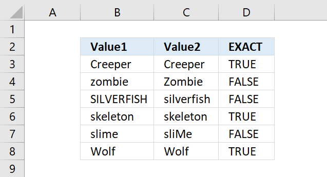
The EXACT function compares value to value and returns boolean values TRUE or FALSE, the above image shows the EXACT function column D comparing corresponding values on the same row in columns B and C.
Formula in cell D3:
Cells B3 and C3 contain the exact same value and the EXACT function returns TRUE. Cell B4 contain "zombie" and cell C4 contain "Zombie", the first letters have a different case. The EXACT function returns FALSE.
5. Does the function ignore cell formatting?
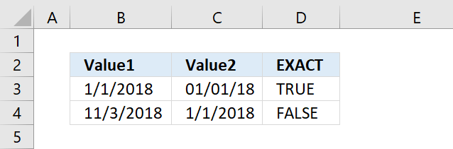
This example demonstrates that cell formatting is ignored. The image above shows two different dates in cells B3, C3, B4, and C4. Cell B3 contains "1/1/2018" and C3 contains "01/01/2018", it is the exact same date, however the latter date shows day and month in two digits whereas the former shows day and month in single digits. It is obviously not an exact match, why is the EXACT function returning TRUE?
The reason is that the cell value contains 43101 in both cells and they are therefore identical but they are also formatted differently. The answer to the question is: Yes, the EXACT function ignores cell formatting differences.
Excel uses whole numbers as dates, in other words, dates are stored as serial numbers. Each date is assigned a sequential integer value starting from 1/1/1900 as serial #1.
Serial numbers represent elapsed days, the integer values represent the number of elapsed days since January 1st, 1900. This allows easy date calculations in Excel.
Excel formats cells as dates automatically if you type valid dates, however, they are stored as numbers. You can verify this by changing formatting from date to general, this shows the number representing the date.
6. How to perform a case sensitive count based on a condition

The formula in cell F2 counts cells in cell range B3:B12 based on the condition specified in cell D3, the count is case sensitive.
The result is 2, cells B3 and B11 equal the condition in cell D3.
Formula in cell F3:
Explaining formula in cell F3
Step 1 - Identify cells equal to condition case sensitive
EXACT(D3,B3,B12)
becomes
EXACT("R",{"R"; "W"; "r"; "I"; "r"; "W"; "H"; "W"; "R"; "O"})
and returns
{TRUE; FALSE; FALSE; FALSE; FALSE; FALSE; FALSE; FALSE; TRUE; FALSE}.
Step 2 - Multiply with 1
The SUMPRODUCT function can't add boolean values, we need to convert them to their numerical equivalents.
The asterisk character lets you multiply values in Excel formulas.
EXACT(D3,B3,B12)*1
becomes
{TRUE; FALSE; FALSE; FALSE; FALSE; FALSE; FALSE; FALSE; TRUE; FALSE}*1
and returns
{1; 0; 0; 0; 0; 0; 0; 0; 1; 0}.
Step 3 - Sum values
The SUMPRODUCT function adds values and returns a total, the reason we don't use the SUM function is that it requires us to enter the formula as an array formula.
SUMPRODUCT(EXACT(D3,B3,B12)*1)
becomes
SUMPRODUCT({1; 0; 0; 0; 0; 0; 0; 0; 1; 0})
and returns 2.
7. Calculate average based on a case sensitive condition

Array formula in cell G3:
7.1 How to enter an array formula

The image above shows a leading and trailing curly bracket. They appear automatically when you follow the steps below.
- Copy the array formula above.
- Double press with the left mouse button on cell G3, a prompt appears.
- Paste the formula to cell G3, shortcut keys are CTRL + v.
- Press and hold CTRL + SHIFT keys simultaneously.
- Press Enter once.
- Release all keys.
The formula bar shows a beginning and ending curly bracket, don't enter these characters yourself.
7.2 Explaining formula
Step 1 - Compare condition to values also considering capital and lower letters
EXACT(E3, B3:B12)
becomes
EXACT("R", {"R"; "W"; "r"; "I"; "r"; "R"; "H"; "W"; "R"; "O"})
and returns
{TRUE; FALSE; FALSE; FALSE; FALSE; TRUE; FALSE; FALSE; TRUE; FALSE}.
Step 2 - Replace TRUE with corresponding value on the same row
The IF function returns one value if the logical test is TRUE and another value if the logical test is FALSE.
IF(logical_test, [value_if_true], [value_if_false])
IF(EXACT(E3,B3:B12), C3:C12, "")
beomes
IF({TRUE; FALSE; FALSE; FALSE; FALSE; TRUE; FALSE; FALSE; TRUE; FALSE}, C3:C12, "")
becomes
IF({TRUE; FALSE; FALSE; FALSE; FALSE; TRUE; FALSE; FALSE; TRUE; FALSE}, {69; 67; 81; 16; 80; 17; 98; 37; 16; 80}, "")
and returns
{69; ""; ""; ""; ""; 17; ""; ""; 16; ""}.
Step 3 - Calculate the average
The AVERAGE function calculates the average based on a given set of numbers.
AVERAGE(number1, [number2], ...)
AVERAGE(IF(EXACT(E3,B3:B12),C3:C12,""))
becomes
AVERAGE({69; ""; ""; ""; ""; 17; ""; ""; 16; ""})
and returns 34. 69 + 17 + 16 = 102. 102/3 = 34.
8. Calculate a sum based on a case sensitive condition

Array formula in cell G3:
8.1 Explaining formula
Step 1 - Compare condition to values also considering capital and lower letters
EXACT(E3, B3:B12)
becomes
EXACT("R", {"R"; "W"; "r"; "I"; "r"; "R"; "H"; "W"; "R"; "O"})
and returns
{TRUE; FALSE; FALSE; FALSE; FALSE; TRUE; FALSE; FALSE; TRUE; FALSE}.
Step 2 - Replace TRUE with corresponding value on the same row
The IF function returns one value if the logical test is TRUE and another value if the logical test is FALSE.
IF(logical_test, [value_if_true], [value_if_false])
IF(EXACT(E3,B3:B12), C3:C12, "")
beomes
IF({TRUE; FALSE; FALSE; FALSE; FALSE; TRUE; FALSE; FALSE; TRUE; FALSE}, C3:C12, "")
becomes
IF({TRUE; FALSE; FALSE; FALSE; FALSE; TRUE; FALSE; FALSE; TRUE; FALSE}, {69; 67; 81; 16; 80; 17; 98; 37; 16; 80}, "")
and returns
{69; ""; ""; ""; ""; 17; ""; ""; 16; ""}.
Step 3 - Calculate the sum
The SUM function calculates a total.
SUM(number1, [number2], ...)
SUM(IF(EXACT(E3,B3:B12),C3:C12,""))
becomes
SUM({69; ""; ""; ""; ""; 17; ""; ""; 16; ""})
and returns 102. 69 + 17 + 16 = 102.
9. Calculate median based on a case sensitive condition

Array formula in cell G3:
9.1 Explaining formula
Step 1 - Compare condition to values also considering capital and lower letters
EXACT(E3, B3:B12)
becomes
EXACT("R", {"R"; "W"; "r"; "I"; "r"; "R"; "H"; "W"; "R"; "O"})
and returns
{TRUE; FALSE; FALSE; FALSE; FALSE; TRUE; FALSE; FALSE; TRUE; FALSE}.
Step 2 - Replace TRUE with corresponding value on the same row
The IF function returns one value if the logical test is TRUE and another value if the logical test is FALSE.
IF(logical_test, [value_if_true], [value_if_false])
IF(EXACT(E3,B3:B12), C3:C12, "")
beomes
IF({TRUE; FALSE; FALSE; FALSE; FALSE; TRUE; FALSE; FALSE; TRUE; FALSE}, C3:C12, "")
becomes
IF({TRUE; FALSE; FALSE; FALSE; FALSE; TRUE; FALSE; FALSE; TRUE; FALSE}, {69; 67; 81; 16; 80; 17; 98; 37; 16; 80}, "")
and returns
{69; ""; ""; ""; ""; 17; ""; ""; 16; ""}.
Step 3 - Calculate the median
The MEDIAN function calculates the median based on a group of numbers. The median is the middle number of a group of numbers.
MEDIAN(number1, [number2], ...)
MEDIAN(IF(EXACT(E3,B3:B12),C3:C12,""))
becomes
MEDIAN({69; ""; ""; ""; ""; 17; ""; ""; 16; ""})
and returns 17.
10. Case sensitive condition not equal to

The formula in cell F2 counts cells in cell range B3:B12 if not equal to the condition specified in cell D3, the count is case sensitive.
Formula in cell F3:
Explaining formula in cell F3
Step 1 - Identify cells equal to condition case sensitive
EXACT(D3,B3,B12)
becomes
EXACT("R",{"R"; "W"; "r"; "I"; "r"; "W"; "H"; "W"; "R"; "O"})
and returns
{TRUE; FALSE; FALSE; FALSE; FALSE; FALSE; FALSE; FALSE; TRUE; FALSE}.
Step 2 - Change TRUE to FALSE and vice versa
The NOT function returns the boolean opposite to the given argument.
NOT(EXACT(D3,B3,B12))
becomes
NOT({TRUE; FALSE; FALSE; FALSE; FALSE; FALSE; FALSE; FALSE; TRUE; FALSE})
and returns
{FALSE; TRUE; TRUE; TRUE; TRUE; TRUE; TRUE; TRUE; FALSE; TRUE}.
Step 3 - Multiply with 1
The SUMPRODUCT function can't add boolean values, we need to convert them to their numerical equivalents.
The asterisk character lets you multiply values in Excel formulas.
NOT(EXACT(D3,B3,B12))*1
becomes
{FALSE; TRUE; TRUE; TRUE; TRUE; TRUE; TRUE; TRUE; FALSE; TRUE}*1
and returns
{0; 1; 1; 1; 1; 1; 1; 1; 0; 1}.
Step 4 - Sum values
The SUMPRODUCT function adds values and returns a total, the reason we don't use the SUM function is that it requires us to enter the formula as an array formula.
SUMPRODUCT(EXACT(D3,B3,B12)*1)
becomes
SUMPRODUCT({0; 1; 1; 1; 1; 1; 1; 1; 0; 1})
and returns 8.
11. Function not working
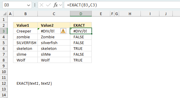
The EXACT function
- propagates errors meaning the function returns an error if an error exists in the source data range.
- returns a #NAME! error if the function name is misspelled.
11.1 Troubleshooting the error value
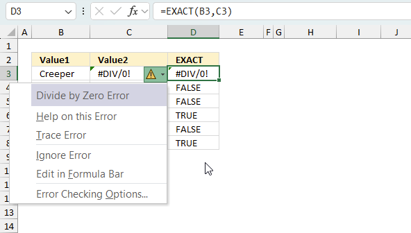
When you encounter an error value in a cell a warning symbol appears, displayed in the image above. Press with mouse on it to see a pop-up menu that lets you get more information about the error.
- The first line describes the error if you press with left mouse button on it.
- The second line opens a pane that explains the error in greater detail.
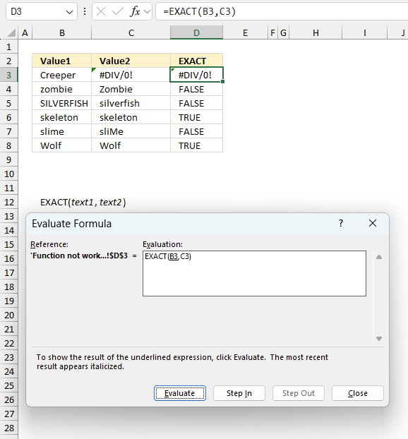
- The third line takes you to the "Evaluate Formula" tool, a dialog box appears allowing you to examine the formula in greater detail.
- This line lets you ignore the error value meaning the warning icon disappears, however, the error is still in the cell.
- The fifth line lets you edit the formula in the Formula bar.
- The sixth line opens the Excel settings so you can adjust the Error Checking Options.
Here are a few of the most common Excel errors you may encounter.
#NULL error - This error occurs most often if you by mistake use a space character in a formula where it shouldn't be. Excel interprets a space character as an intersection operator. If the ranges don't intersect an #NULL error is returned. The #NULL! error occurs when a formula attempts to calculate the intersection of two ranges that do not actually intersect. This can happen when the wrong range operator is used in the formula, or when the intersection operator (represented by a space character) is used between two ranges that do not overlap. To fix this error double check that the ranges referenced in the formula that use the intersection operator actually have cells in common.
#SPILL error - The #SPILL! error occurs only in version Excel 365 and is caused by a dynamic array being to large, meaning there are cells below and/or to the right that are not empty. This prevents the dynamic array formula expanding into new empty cells.
#DIV/0 error - This error happens if you try to divide a number by 0 (zero) or a value that equates to zero which is not possible mathematically.
#VALUE error - The #VALUE error occurs when a formula has a value that is of the wrong data type. Such as text where a number is expected or when dates are evaluated as text.
#REF error - The #REF error happens when a cell reference is invalid. This can happen if a cell is deleted that is referenced by a formula.
#NAME error - The #NAME error happens if you misspelled a function or a named range.
#NUM error - The #NUM error shows up when you try to use invalid numeric values in formulas, like square root of a negative number.
#N/A error - The #N/A error happens when a value is not available for a formula or found in a given cell range, for example in the VLOOKUP or MATCH functions.
#GETTING_DATA error - The #GETTING_DATA error shows while external sources are loading, this can indicate a delay in fetching the data or that the external source is unavailable right now.
11.2 The formula returns an unexpected value
To understand why a formula returns an unexpected value we need to examine the calculations steps in detail. Luckily, Excel has a tool that is really handy in these situations. Here is how to troubleshoot a formula:
- Select the cell containing the formula you want to examine in detail.
- Go to tab “Formulas” on the ribbon.
- Press with left mouse button on "Evaluate Formula" button. A dialog box appears.
The formula appears in a white field inside the dialog box. Underlined expressions are calculations being processed in the next step. The italicized expression is the most recent result. The buttons at the bottom of the dialog box allows you to evaluate the formula in smaller calculations which you control. - Press with left mouse button on the "Evaluate" button located at the bottom of the dialog box to process the underlined expression.
- Repeat pressing the "Evaluate" button until you have seen all calculations step by step. This allows you to examine the formula in greater detail and hopefully find the culprit.
- Press "Close" button to dismiss the dialog box.
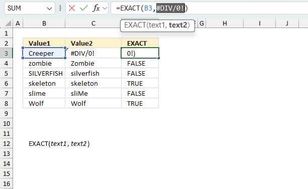
There is also another way to debug formulas using the function key F9. F9 is especially useful if you have a feeling that a specific part of the formula is the issue, this makes it faster than the "Evaluate Formula" tool since you don't need to go through all calculations to find the issue..
- Enter Edit mode: Double-press with left mouse button on the cell or press F2 to enter Edit mode for the formula.
- Select part of the formula: Highlight the specific part of the formula you want to evaluate. You can select and evaluate any part of the formula that could work as a standalone formula.
- Press F9: This will calculate and display the result of just that selected portion.
- Evaluate step-by-step: You can select and evaluate different parts of the formula to see intermediate results.
- Check for errors: This allows you to pinpoint which part of a complex formula may be causing an error.
The image above shows cell reference C3 converted to hard-coded value using the F9 key. The EXACT function requires valid non-error values which is not the case in this example. We have found what is wrong with the formula.
Tips!
- View actual values: Selecting a cell reference and pressing F9 will show the actual values in those cells.
- Exit safely: Press Esc to exit Edit mode without changing the formula. Don't press Enter, as that would replace the formula part with the calculated value.
- Full recalculation: Pressing F9 outside of Edit mode will recalculate all formulas in the workbook.
Remember to be careful not to accidentally overwrite parts of your formula when using F9. Always exit with Esc rather than Enter to preserve the original formula. However, if you make a mistake overwriting the formula it is not the end of the world. You can “undo” the action by pressing keyboard shortcut keys CTRL + z or pressing the “Undo” button
11.3 Other errors
Floating-point arithmetic may give inaccurate results in Excel - Article
Floating-point errors are usually very small, often beyond the 15th decimal place, and in most cases don't affect calculations significantly.
Useful links
EXACT function - Microsoft support
EXACT Function in Excel: Explained
'EXACT' function examples

First, let me explain the difference between unique values and unique distinct values, it is important you know the difference […]

This post explains how to lookup a value and return multiple values. No array formula required.
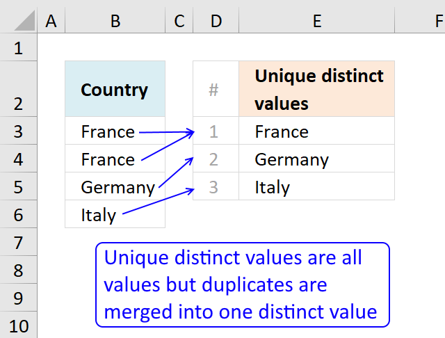
This article describes how to count unique distinct values. What are unique distinct values? They are all values but duplicates are […]
Functions in 'Text' category
The EXACT function function is one of 29 functions in the 'Text' category.
How to comment
How to add a formula to your comment
<code>Insert your formula here.</code>
Convert less than and larger than signs
Use html character entities instead of less than and larger than signs.
< becomes < and > becomes >
How to add VBA code to your comment
[vb 1="vbnet" language=","]
Put your VBA code here.
[/vb]
How to add a picture to your comment:
Upload picture to postimage.org or imgur
Paste image link to your comment.
Contact Oscar
You can contact me through this contact form