Compare two columns in different worksheets

This article describes an array formula that compares values from two different columns in two worksheets twice and returns a value if criteria are met.
What's on this page
- Compare two columns in different worksheets
- Compare two columns in different worksheets (Excel 2016)
- Get Excel file
- Compare two columns and return differences
- Compare two columns and return differences sorted from A to Z
- Compare two columns and return differences - Excel 365
- Compare two columns and return differences sorted from A to Z - Excel 365
- Extract values that exist only in one of the two columns
- Extract values that exist only in one of the two columns - Excel 365
- Identify missing numbers in a range
- Filter values occurring in range 1 but not in range 2
- Filter not shared values out of two cell ranges - UDF
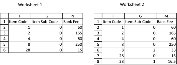
There are multiple columns in two different worksheets, one has more columns than another. I need to compare column F of worksheet 1 and column E of worksheet 2; if the value matches, compare column G of worksheet 1 and column F of worksheet 2; if the value matches, record the value in column N of worksheet1 from column M of worksheet 2. Please see the example below.
Worksheet 1:
Column F Column G Column N
Item Code Item Sub-Code Bank Fee
1 0
2 0
4 0
8 0
28 0
Worksheet2:
Column E Column F Column M
Item Code Item Sub-Code Bank Fee
1 0 60
2 0 165
4 0 60
8 0 250
8 2 33
28 0 15
28 1 16.5
Appreciate your help in advance!
Array formula in cell N2, worksheet 1:
1.1 How to enter an array formula
- Copy and paste the formula above to cell N2.
- Press and hold CTRL + SHIFT simultaneously.
- Press Enter once.
- Release all keys.
The formula is now surrounded by curly brackets, like this {=formula} if you did it right. Check your formula bar and make sure you have the curly brackets.
Then copy cell N2 and paste to cells below.
1.2 Explaining array formula in cell N2
Step 1 - Compare cell F2 (sheet1) with column F (sheet2)
The equal sign is a logical operator that allows you to compare values. It also allows you to compare a value to multiple values, this returns an array of values.
F2=Sheet2!$F$2:$F$8 returns {TRUE; FALSE; FALSE; ...; FALSE}
TRUE and FALSE are boolean values.
Step 2 - Compare cell G2 (sheet1) with column G (sheet2)
G2=Sheet2!$G$2:$G$8 returns {TRUE; TRUE; TRUE; ... ; FALSE}
Step 3 - Multiply arrays
This step multiples both arrays to apply AND-logic meaning both boolean values must be TRUE in order to return TRUE. See all possible combinations below.
TRUE * TRUE = TRUE (1)
TRUE * FALSE = FALSE (0)
FALSE * TRUE = FALSE (0)
FALSE * FALSE = FALSE (0)
(F2=Sheet2!$F$2:$F$8)*(Sheet1!G2=Sheet2!$G$2:$G$8) returns {1; 0; 0; 0; 0; 0; 0}.
The calculation returns the numerical equivalent to the boolean values, TRUE returns 1, and FALSE returns 0 (zero).
Step 4 - Use IF function to replace calculated values with sheet2 values from column N, if TRUE (1)
The IF function returns one value if the logical test is TRUE and another value if the logical test is FALSE.
IF(logical_test, [value_if_true], [value_if_false])
IF((F2=Sheet2!$F$2:$F$8)*(Sheet1!G2=Sheet2!$G$2:$G$8), Sheet2!$N$2:$N$8, "") returns {60; ""; ""; ""; ""; ""; ""}.
Step 5 - Calculate the smallest number in the array
The MIN function returns the smallest number in an array or cell range, it ignores logical and text values
MIN(IF((F2=Sheet2!$F$2:$F$8)*(Sheet1!G2=Sheet2!$G$2:$G$8), Sheet2!$N$2:$N$8, ""))
becomes MIN({60;"";"";"";"";"";""}) and returns 60.
2. Compare two columns in different worksheets (Excel 2016)

Excel 2016 formula in cell N2:
Explaining formula in cell N2
Step 1 - Setup MINIFS function
The MINIFS function calculates the smallest value based on a given set of criteria.
MINIFS(min_range, criteria_range1, criteria1, [criteria_range2, criteria2], ...)
MINIFS(Sheet2!$N$2:$N$8, Sheet2!$F$2:$F$8, F2, Sheet2!$G$2:$G$8, G2)
Step 2 - Evaluate MINIFS function
MINIFS(Sheet2!$N$2:$N$8, Sheet2!$F$2:$F$8, F2, Sheet2!$G$2:$G$8, G2)
becomes MINIFS({60;165;60;250;33;15;16.5},{1;2;4;8;8;28;28},1,{0;0;0;0;2;0;1},0)
and returns 60. The only relative position that meets both criteria is the first one, it contains number 60.
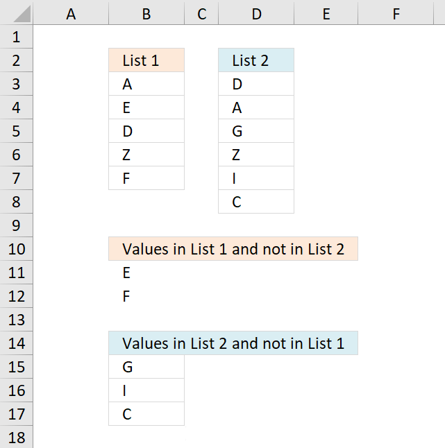
This section demonstrates formulas that extract differences between two given lists. The first formula in cell B11 extracts values from List 1 that doesn't exist in List 2. The second formula in cell B15 extracts values from List 2 that is not in List 1.
4. Compare two columns and return differences
The image above demonstrates an array formula in cell B11 that extracts values that only exist in List 1 (B3:B7) and not in List 2 (D3:D8). The same formula is used in cell B15, however, with different cell references. This time it extracts values that only exist in List 2 (D3:D8).
Array Formula in B11:
To enter an array formula press and hold CTRL + SHIFT simultaneously, then press Enter once. Release all keys.
The formula bar now shows the formula enclosed with curly brackets telling you that you entered the formula successfully. Don't enter the curly brackets yourself.
Copy cell D2 and paste it down as far as needed.
Array Formula in B15:
Copy cell D9 and paste it down as far as needed.
Explaining formula in cell B11
Step 1 - Count values in List 1 based on values in List 1
The COUNTIF function counts values based on a condition or criteria.
COUNTIF($D$3:$D$8, $B$3:$B$7)=0 returns {FALSE; TRUE; FALSE; FALSE; TRUE}
Step 2 - Replace TRUE with corresponding row number
The IF function has three arguments, the first one must be a logical expression. If the expression evaluates to TRUE then one thing happens (argument 2) and if FALSE another thing happens (argument 3).
IF(COUNTIF($D$3:$D$8, $B$3:$B$7)=0, MATCH(ROW($B$3:$B$7), ROW($B$3:$B$7)), "") returns {""; 2; ""; ""; 5}
Step 3 - Extract k-th smallest row number
To be able to return a new value in a cell each I use the SMALL function to filter row numbers from smallest to largest.
The ROWS function keeps track of the numbers based on an expanding cell reference. It will expand automatically when the cell is copied to the cells below.
SMALL(IF(COUNTIF($B$3:$B$7, $D$3:$D$8)=0, MATCH(ROW($D$3:$D$8), ROW($D$3:$D$8)),""), ROWS($A$1:A1)) returns 2.
Step 4 - Get value
The INDEX function returns a value based on a cell reference and a row number (also a column number if needed).
INDEX($D$3:$D$8, SMALL(IF(COUNTIF($B$3:$B$7, $D$3:$D$8)=0, MATCH(ROW($D$3:$D$8), ROW($D$3:$D$8)),""), ROWS($A$1:A1))) returns "E" in cell B11.
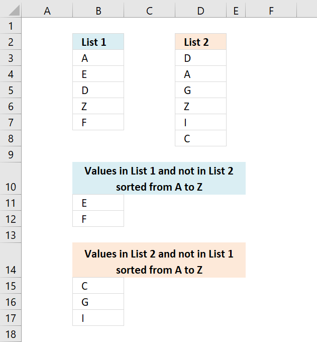
5. Compare two columns and return differences sorted from A to Z
Array Formula in B11:
Array Formula in B15:
6. Compare two columns and return differences - Excel 365
The formula in cell B11 works only in Excel 365, it contains the new FILTER function. It filters values in list 1 that only exists in list 1 compared to list 2.
Excel 365 dynamic array formula in cell B11:
The formula in cell B15 filters values in list 2 that only exists in list 2 compared to list 1.
Excel 365 dynamic array formula in cell B15:
6.1 Explaining formula in cell B11
Step 1 - Count values in D3:D8 based on criteria in B3:B7
The COUNTIF function calculates the number of cells that is equal to a condition.
Function syntax: COUNTIF(range, criteria)
COUNTIF(D3:D8, B3:B7) returns {1; 0; 1; 1; 0}
Step 2 - Check if a value in the array is equal to 0 (zero)
The equal sign lets you compare value to value, the result is a boolean value TRUE or FALSE.
COUNTIF(D3:D8, B3:B7)=0 returns {FALSE; TRUE; FALSE; FALSE; TRUE}.
Step 3 - Filter values not in both lists
The FILTER function extracts values/rows based on a condition or criteria.
Function syntax: FILTER(array, include, [if_empty])
FILTER(B3:B7, COUNTIF(D3:D8, B3:B7)=0) returns {"E"; "F"}.
6.2 Explaining formula in cell B15
Step 1 - Count values in B3:B7 based on criteria in D3:D8
The COUNTIF function calculates the number of cells that is equal to a condition.
Function syntax: COUNTIF(range, criteria)
COUNTIF(B3:B7, D3:D8) returns {1; 1; 0; 1; 0; 0}
Step 2 - Check if a value in the array is equal to 0 (zero)
The equal sign lets you compare value to value, the result is a boolean value TRUE or FALSE.
COUNTIF(B3:B7, D3:D8)=0 returns {FALSE; FALSE; TRUE; FALSE; TRUE; TRUE}.
Step 3 - Filter values not in both lists
The FILTER function extracts values/rows based on a condition or criteria.
Function syntax: FILTER(array, include, [if_empty])
FILTER(D3:D8, COUNTIF(B3:B7, D3:D8)=0) returns {"G"; "I"; "C"}.
7. Compare two columns and return differences sorted from A to Z - Excel 365
Excel 365 dynamic array formula in cell B11:
Excel 365 dynamic array formula in cell B15:
7.1 Explaining formula in cell B11
Step 1 - Count values in D3:D8 based on criteria in B3:B7
The COUNTIF function calculates the number of cells that is equal to a condition.
Function syntax: COUNTIF(range, criteria)
COUNTIF(D3:D8, B3:B7) returns {1; 0; 1; 1; 0}
Step 2 - Check if a value in the array is equal to 0 (zero)
The equal sign lets you compare value to value, the result is a boolean value TRUE or FALSE.
COUNTIF(D3:D8, B3:B7)=0 returns {FALSE; TRUE; FALSE; FALSE; TRUE}.
Step 3 - Filter values not in both lists
The FILTER function extracts values/rows based on a condition or criteria.
Function syntax: FILTER(array, include, [if_empty])
FILTER(B3:B7, COUNTIF(D3:D8, B3:B7)=0) returns {"E"; "F"}.
Step 4 - Sort values from A to Z
The SORT function sorts values from a cell range or array
Function syntax: SORT(array,[sort_index],[sort_order],[by_col])
SORT(FILTER(B3:B7, COUNTIF(D3:D8, B3:B7)=0)) returns {"E"; "F"}.
7.2 Explaining formula in cell B15
Step 1 - Count values in B3:B7 based on criteria in D3:D8
The COUNTIF function calculates the number of cells that is equal to a condition.
Function syntax: COUNTIF(range, criteria)
COUNTIF(B3:B7, D3:D8) returns {1; 1; 0; 1; 0; 0}
Step 2 - Check if a value in the array is equal to 0 (zero)
The equal sign lets you compare value to value, the result is a boolean value TRUE or FALSE.
COUNTIF(B3:B7, D3:D8)=0 returns {FALSE; FALSE; TRUE; FALSE; TRUE; TRUE}.
Step 3 - Filter values not in both lists
The FILTER function extracts values/rows based on a condition or criteria.
Function syntax: FILTER(array, include, [if_empty])
FILTER(D3:D8, COUNTIF(B3:B7, D3:D8)=0) returns {"G"; "I"; "C"}.
Step 4 - Sort values from A to Z
The SORT function sorts values from a cell range or array
Function syntax: SORT(array,[sort_index],[sort_order],[by_col])
SORT(FILTER(D3:D8, COUNTIF(B3:B7, D3:D8)=0)) returns {"C", "G"; "I"}.
8. Extract values that exist only in one of two nonadjacent columns
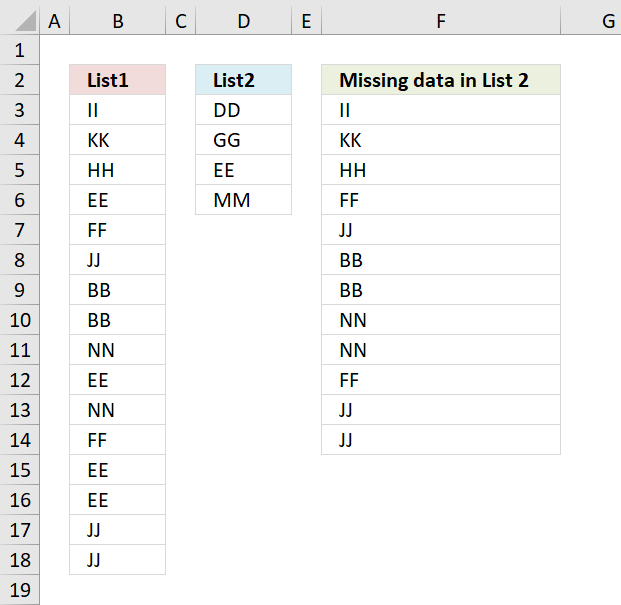
Question: How to filter out data from List 1 that is missing in list 2?
Answer: This formula is useful when comparing two lists to find out what cell values are missing.For instance, inventory comparison.
How to create an array formula
- Select cell c2
- Press with left mouse button on in formula bar
- Paste above array formula to formula bar

- Press and hold Ctrl + Shift
- Press Enter
- Release all keys
You know you have entered an array formula when the formula in the formula bar is surrounded by curly brackets {=array_formula}
Explaining formula
Step 1 - Compare values between A2:A17 and B2:B5
 The MATCH function looks for a specific value in a cell range or array and returns it's position in that cell range or array.
If the value does not exist in the cell range or array the MATCH function returns #N/A (error value).
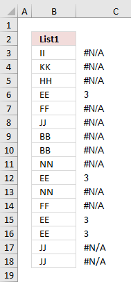
MATCH($A$2:$A$17, $B$2:$B$5, 0)
checks if there are any matches. If there are none, an error will occur.
{#N/A,#N/A,... ,#N/A,}
The image to the right shows the array and the corresponding value in column B. It is quite obvious already now which values are missing in the List 2 and which ones that exist.
Step 2 - Identify error values in array
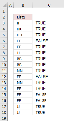 If a value in array is an error the ISERROR function returns TRUE else FALSE.
ISERROR(MATCH($A$2:$A$17, $B$2:$B$5, 0))
returns {TRUE, TRUE, ... , TRUE, }
The array now contains boolean values, TRUE or FALSE.
The IF function in the next step can't handle error values so this step is necessary.
Step 3 - Convert boolean value TRUE to the corresponding row number
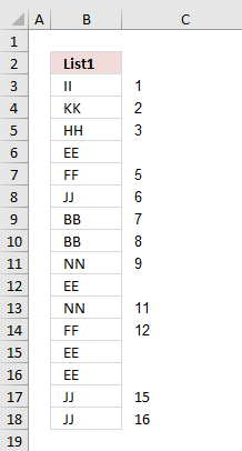 The IF function allows you to specify a logical expression and if it evaluates to TRUE one thing happens and if FALSE another thing happens.
IF(ISERROR(MATCH($A$2:$A$17, $B$2:$B$5, 0)), (ROW($A$2:$A$17)-MIN(ROW($A$2:$A$17))+1), "")
returns {1,2,3,4,"",6,7,8,9,"",11,12,"","",15,16}
If there is an error in the array, replace that error with the row number.
Step 4 - Return the k-th smallest row number
In this example one cell will display one value and in order to do that the small function returns a single row number for each cell allowing you to get a single value in each cell.
SMALL(IF(ISERROR(MATCH($A$2:$A$17, $B$2:$B$5, 0)), (ROW($A$2:$A$17)-MIN(ROW($A$2:$A$17))+1), ""), ROW(1:1))
becomes
SMALL({1,2,3,4,"",6,7,8,9,"",11,12,"","",15,16}, 1)
and returns 1.
Step 5 - Use the row number to get the correct value
The INDEX function allows you to get a value based on a row number and column number.
INDEX($A$2:$A$17, SMALL(IF(ISERROR(MATCH($A$2:$A$17, $B$2:$B$5, 0)), (ROW($A$2:$A$17)-MIN(ROW($A$2:$A$17))+1), ""), ROW(1:1)))
returns II in cell C2.
9. Extract values that exist only in one of two nonadjacent columns - Excel 365

The image above demonstrates an Excel 365 formula much smaller than the above, it also extracts missing values between two nonadjacent columns.
Formula in cell F3:
2.1 Explaining formula
Step 1 - Count cells equal to any of the conditions
The COUNTIF function calculates the number of cells that meet a given condition.
COUNTIF(range, criteria)
COUNTIF(D3:D6, B3:B18)
returns {0; 0; ... ; 0}
Step 2 - Check if value in the array is equal to 0 (zero)
The equal sign lets you check if a value is equal to another value. The result is a boolean value, TRUE or FALSE.
COUNTIF(D3:D6,B3:B18)=0
returns {TRUE; TRUE; ... ; TRUE}
Step 3 - Filter values based on boolean values
FILTER(B3:B18,COUNTIF(D3:D6,B3:B18)=0)
returns {"II"; "KK"; ... ; "JJ"}.
10. Identify missing numbers in a range
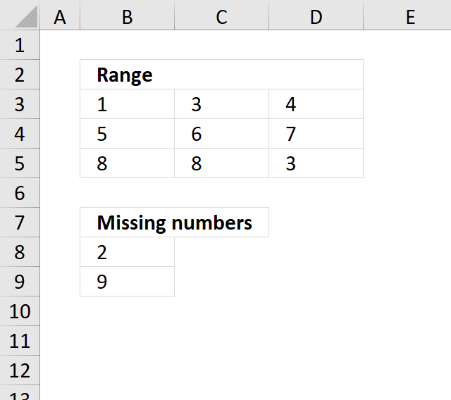
Question: How do I find missing numbers between 1-9 in a range?
1 3 4
5 6 7
8 8 3
Array formula in cell B8:
If you have numbers between 5 and 32, change ROW($1:$9) to ROW($5:$32)
The formula won´t work if you have numbers above 1048576 (excel 2007). See this post: Identify missing values in a column using excel formula
How to create an array formula
- Copy above array formula
- Select cell B8
- Press with left mouse button on in formula bar
- Paste array formula in formula bar
- Press and hold Ctrl + Shift
- Press Enter
Explaining formula in cell B8
Step 1 - Check if numbers in range equal numbers in list
The COUNTIF function counts values based on a condition, in this case, multiple conditions. The first argument is the cell range containing the numbers, the second argument is a given list of numbers.
The ROW function returns the row number of a cell, in this case a cell range. The ROW function then returns an array of row numbers of all cells in the cell range.
COUNTIF($B$3:$D$5, ROW($1:$9)
returns {1;0;2;1;1;1;1;2;0}.
Step 2 - Which numbers are missing?
A 0 (zero) indicates a number is missing, compare the value with 0 (zero) and we get either TRUE or FALSE.
COUNTIF($B$3:$D$5,ROW($1:$9))=0
returns {FALSE; ... ; TRUE}.
Step 3 - Replace TRUE with corresponding number
IF(COUNTIF($B$3:$D$5, ROW($1:$9))=0, ROW($1:$9), "")
returns {"";2;"";"";"";"";"";"";9}.
Step 4 - Extract a new number in a cell each
The SMALL function extracts the k-th smallest number from a cell range or array. SMALL( cell_ref, k)
The second argument contains the ROWS function and an expanding cell range. When you copy the cell and paste to cells below the cell reference grows. This makes sure that a new numb er is extracted in each cell.
SMALL(IF(COUNTIF($B$3:$D$5, ROW($1:$9))=0, ROW($1:$9), ""), ROWS(B8:$B$8)
becomes SMALL({"";2;"";"";"";"";"";"";9}, 1) and returns 2 in cell B8.
Get Excel *.xls file
Missing numbers in a range.xls
11. Filter values occurring in range 1 but not in range 2
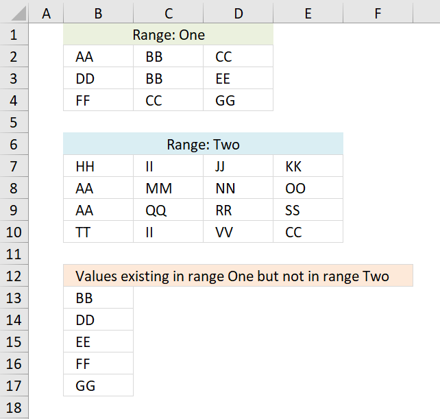
The formulas above extracts values that exists only in one or the other cell range, if you are looking for a formula that compares two separate columns the go here: Compare two columns and show differences
Excel 365 formula in cell B13:
Array formula in B13:
Array formula in B22:
To enter an array formula, type the formula in a cell then press and hold CTRL + SHIFT simultaneously, now press Enter once. Release all keys.
The formula bar now shows the formula with a beginning and ending curly bracket telling you that you entered the formula successfully. Don't enter the curly brackets yourself.
If you don't own an Excel version that has the TEXTJOIN function then use the following considerably larger formula.
Array formula in B13:
copied down as far as necessary.
Formula in B21:
copied down as far as necessary.
Explaining formula in cell B13
Step 1 - Identify values not shared by the ranges
The COUNTIF function counts values based on a condition or criteria, in this case, it counts values between the cell ranges.
COUNTIF($B$7:$E$10, $B$2:$D$4)=0
becomes
COUNTIF({"HH", "II", "JJ", "KK";"AA", "MM", "NN", "OO";"AA", "QQ", "RR", "SS";"TT", "II", "VV", "CC"}, {"AA", "BB", "CC";"DD", "BB", "EE";"FF", "CC", "GG"})=0
becomes
{2,0,1;0,0,0;0,1,0}=0
and returns
{FALSE, TRUE, FALSE;TRUE, TRUE, TRUE;TRUE, FALSE, TRUE}.
Step 2 - Prevent duplicates in list
COUNTIF(B12:$B$12, $B$2:$D$4)
becomes
COUNTIF("Values existing in range One but not in range Two", {"AA", "BB", "CC";"DD", "BB", "EE";"FF", "CC", "GG"})
and returns
{0,0,0;0,0,0;0,0,0}.
Step 3 - Add arrays
Check if array is equal to 1.
((COUNTIF($B$7:$E$10, $B$2:$D$4)=0)+COUNTIF(B12:$B$12, $B$2:$D$4))=1
becomes
({FALSE, TRUE, FALSE;TRUE, TRUE, TRUE;TRUE, FALSE, TRUE}+{0,0,0;0,0,0;0,0,0})=1
becomes
{0,1,0;1,1,1;1,0,1}=1
and returns
{FALSE,TRUE,FALSE;TRUE,TRUE,TRUE;TRUE,FALSE,TRUE}.
Step 4 - Convert TRUE to a unique number
IF(((COUNTIF($B$7:$E$10, $B$2:$D$4)=0)+COUNTIF(B12:$B$12, $B$2:$D$4))=1, (ROW($B$2:$D$4)+(1/(COLUMN($B$2:$D$4)+1)))*1, "")
becomes
IF({FALSE, TRUE, FALSE;TRUE, TRUE, TRUE;TRUE, FALSE, TRUE}, (ROW($B$2:$D$4)+(1/(COLUMN($B$2:$D$4)+1)))*1, "")
becomes
IF({FALSE, TRUE, FALSE;TRUE, TRUE, TRUE;TRUE, FALSE, TRUE}, {2.33333333333333, 2.25, 2.2;3.33333333333333, 3.25, 3.2;4.33333333333333, 4.25, 4.2}, "")
and returns
{"", 2.25, "";3.33333333333333, 3.25, 3.2;4.33333333333333, "", 4.2}
Step 5 - Find smallest number in array
The MIN function returns the minimum number in the given array.
MIN(IF(((COUNTIF($B$7:$E$10, $B$2:$D$4)=0)+COUNTIF(B12:$B$12, $B$2:$D$4))=1, (ROW($B$2:$D$4)+(1/(COLUMN($B$2:$D$4)+1)))*1, ""))
becomes
MIN({"", 2.25, "";3.33333333333333, 3.25, 3.2;4.33333333333333, "", 4.2})
and returns 2.25
Step 6 - Find position in array
IF(MIN(IF(((COUNTIF($B$7:$E$10, $B$2:$D$4)=0)+COUNTIF(B12:$B$12, $B$2:$D$4))=1, (ROW($B$2:$D$4)+(1/(COLUMN($B$2:$D$4)+1)))*1, ""))=(ROW($B$2:$D$4)+(1/(COLUMN($B$2:$D$4)+1)))*1, $B$2:$D$4, "")
becomes
IF(2.25=(ROW($B$2:$D$4)+(1/(COLUMN($B$2:$D$4)+1)))*1, $B$2:$D$4, "")
becomes
IF(2.25={2.33333333333333, 2.25, 2.2;3.33333333333333, 3.25, 3.2;4.33333333333333, 4.25, 4.2}, $B$2:$D$4, "")
and returns {"","BB","";"","","";"","",""}.
Step 7 - Concatenate strings in array
The TEXTJOIN function returns values concatenated ignoring blanks in array.
TEXTJOIN("", TRUE, IF(MIN(IF(((COUNTIF($B$7:$E$10, $B$2:$D$4)=0)+COUNTIF(B12:$B$12, $B$2:$D$4))=1, (ROW($B$2:$D$4)+(1/(COLUMN($B$2:$D$4)+1)))*1, ""))=(ROW($B$2:$D$4)+(1/(COLUMN($B$2:$D$4)+1)))*1, $B$2:$D$4, ""))
becomes
TEXTJOIN("", TRUE, {"","BB","";"","","";"","",""})
and returns "BB" in cell B13.
Get Excel *.xlsx file
Filter values existing in Range 1 but not in Range 2.xlsx
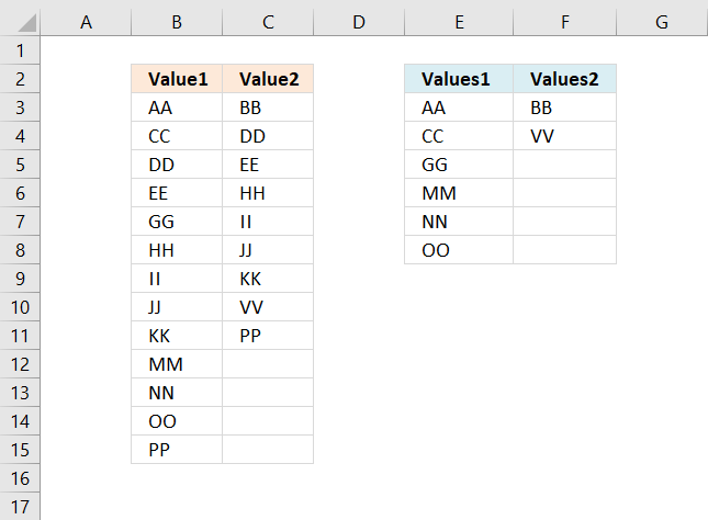
12. Filter not shared values out of two cell ranges - UDF

This post describes a custom function (User defined Function) that extract values existing only in one out of two cell ranges, see picture above. For example, value II is not extracted because it exists in both cell ranges Range1 and Range2.
This UDF is useful if you have lots of data and a formula is too slow.
Array formula in cell range B9:B22:
To enter an array formula, type the formula in a cell then press and hold CTRL + SHIFT simultaneously, now press Enter once. Release all keys.
The formula bar now shows the formula with a beginning and ending curly bracket telling you that you entered the formula successfully. Don't enter the curly brackets yourself.
Excel user defined function
Function Filter_Values(rng1 As Variant, rng2 As Variant) As Variant
' This udf filter values that exists only in one out of two ranges
Dim Value As Variant
Dim temp() As Variant
Dim Test1 As New Collection
Dim Test2 As New Collection
ReDim temp(0)

 rng1 = rng1.Value
 rng2 = rng2.Value

On Error Resume Next
For Each Value In rng1
 If Len(Value) > 0 Then Test1.Add Value, CStr(Value)
Next Value

For Each Value In rng2
 If Len(Value) > 0 Then Test2.Add Value, CStr(Value)
Next Value

Err = False
For Each Value In Test2
 If Len(Value) > 0 Then Test1.Add Value, CStr(Value)
 If Err Then
  Test1.Remove Value
 End If
 Err = False
Next Value

For Each Value In Test1
 temp(UBound(temp)) = Value
 ReDim Preserve temp(UBound(temp) + 1)
Next Value
On Error GoTo 0

Filter_Values = Application.Transpose(temp)

End Function
How to add the User defined Function to your workbook
1. Press Alt-F11 to open visual basic editor
2. Press with left mouse button on Module on the Insert menu
3. Copy and paste the above user defined function
4. Exit visual basic editor
5. Select sheet1
6. Select cell range A1:A5000
7. Type =Filter_Values(Sheet2!A1:J500, Sheet3!A1:J500) into formula bar and press CTRL+SHIFT+ENTER
The excel file contains 5000 random values in each range.
Compare category
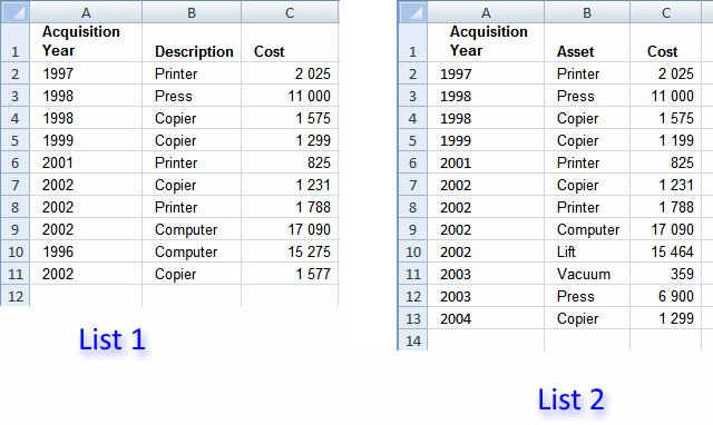
Table of Contents Compare tables: Filter records occurring only in one table Compare two lists and filter unique values where […]
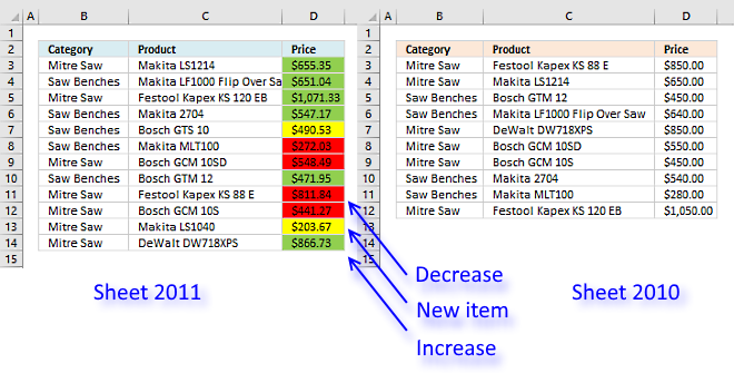
This article demonstrates techniques to highlight differences and common values across lists. What's on this page How to highlight differences […]
This article demonstrates formulas that extract values that exist only in one column out of two columns. There are text […]
Excel categories
14 Responses to “Compare two columns in different worksheets”
Leave a Reply
How to comment
How to add a formula to your comment
<code>Insert your formula here.</code>
Convert less than and larger than signs
Use html character entities instead of less than and larger than signs.
< becomes < and > becomes >
How to add VBA code to your comment
[vb 1="vbnet" language=","]
Put your VBA code here.
[/vb]
How to add a picture to your comment:
Upload picture to postimage.org or imgur
Paste image link to your comment.
I have a worksheet that has rows, each containing sequential groupings of values of "1" and "0" These alternate across 1800 colunms of data.
My question: how do I count the number of groupings of each? In other words, across those 1800 columns, how many arrays of value 1 and how many arrays of value 0 do I have?
Thanks.
Joe
Joe,
see this post:
Count the number of groupings of each value
thanks
How can I expand the range? my list goes til 49
Thank You
Karla,
there are two cell ranges in this formula (bolded):
Change these two cell ranges:
$A$2:$A$17
$B$2:$B$5
Why is it that the formula posted on this web page, is not the same as the formula embedded in the excel document? The formula in the excel document is longer (it has multiple relative cell references, whereas the formula in the excel spreadhseet refers to absolute cell references). If I copy/paste the formula on this page, it does not return any results; it is simply a long formula. Also, when I follow steps on how to create an array formula, it says that a bracket will appear aroun dthe formula, but that did not happen in my case. Any clues appreciated!
Lisa,
Why is it that the formula posted on this web page, is not the same as the formula embedded in the excel document?
I changed the array formula in the post but forgot to change the attached file. Thanks for reminding me.
The formula in the excel document is longer (it has multiple relative cell references, whereas the formula in the excel spreadhseet refers to absolute cell references)
The array formula shown in this post is easier to use, you simply change the absolute cell references in the array formula.
If I copy/paste the formula on this page, it does not return any results; it is simply a long formula. Also, when I follow steps on how to create an array formula, it says that a bracket will appear around the formula, but that did not happen in my case. Any clues appreciated!
Did you paste the formula to the formula bar?
Is there any difference to apply this formula in only one column (F2:F1093)? I´m trying to identify missing numbers in a list but I´m making something wrong.
Felipe,
Did you enter it as an array formula?
Good support and help to improve my excel knowledge.
thanks of lot
Thank you!
How do I combine this function with TEXTJOIN to return all missing values in a single cell, delimited? The current formula I have, which is returning only the first missing value, is:
=arrayformula(Textjoin(" &

", true, (INDEX(Emails!$A$2:$A$36,(MATCH(TRUE,(ISNA(MATCH(Emails!$A$2:$A$36,B$5:B$203,0))),0))))))
This is in google sheets, hence the "arrayformula".
How do I combine this formula with the TEXTJOIN function to return all missing values in a single cell? The formula I currently have, which is returning only the first missing value, is:
=arrayformula(Textjoin(" &", true, (INDEX(Emails!$A$2:$A$36,(MATCH(TRUE,(ISNA(MATCH(Emails!$A$2:$A$36,B$5:B$203,0))),0))))))
This is in google sheets, not excel.
I recently came across a great online tool https://datadiffer.com/ that's perfect for comparing two columns in Excel. Just save the data as txt files and upload them, and you can quickly see what's unique to each file and what's common. It's super easy to use and you can even download the comparison results. It's incredibly handy for anyone who needs to do data analysis!