Count unique distinct values
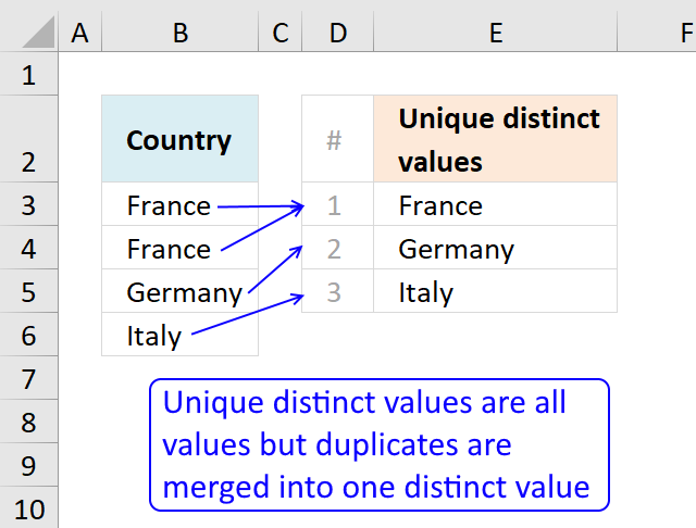
This article describes how to count unique distinct values. What are unique distinct values? They are all values but duplicates are merged into one distinct value.
To count unique distinct records, read this article: Count unique distinct records
You will also find a formula to count unique values, see the table of Contents below. Unique values are values that exist only once in a list or cell range. If a value has a duplicate they are not unique and not counted.
If you are working with lots of data I highly recommend using a pivot table. Excel 2013 and later versions allow you to count unique distinct values.
Table of Contents
Count unique distinct values - Excel 365
- Count unique distinct values - Excel 365
- Count unique distinct values in a cell range with blanks - Excel 365
- Count unique distinct values in multiple nonadjacent cell ranges - Excel 365
- Count unique distinct values
- Count unique distinct values in a cell range with blanks
- Count unique distinct values (case sensitive)
- Count unique distinct values in two columns
- Count unique distinct months
- Count digits and ignore duplicates
- Count unique distinct values in a large dataset - UDF
- Count unique values
- Count unique values (case sensitive)
- Count unique distinct values within same week, month or year
- Introduction
- How to count unique distinct items based on a condition and a date condition - Excel 365?
- How to count unique distinct items based on two conditions and a date condition - Excel 365?
- How to unique distinct products using OR logic - Excel 365?
- Earlier Excel versions
- How to count unique distinct items based on a condition and a date condition?
- How many unique distinct products did Jennifer sell in January and in region South?
- How many unique distinct products was sold in the south or in January?
- Count unique distinct records
- Count records with possible blank rows in data set
- How to count blank rows/records
- Count unique distinct records based on a date and column criteria
- Count unique distinct values based on a condition
- Count unique distinct values based on a condition - Excel 365
- How to count unique distinct values based on a date
Count unique distinct values - earlier Excel versions
Count unique distinct values - User defined function
Count unique values
All Excel versions
Count unique distinct values that meet multiple criteria
Count unique distinct records
1 Count unique distinct values - Excel 365

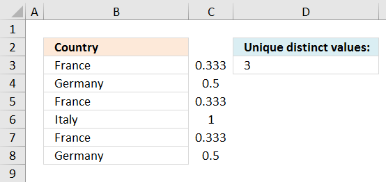
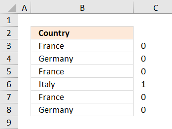
This formula counts unique distinct values in cell range B3:B8, unique distinct values are all values except duplicate values.
For example, the value "France" in cell range B3:B8 has three instances in cells B3, B5, and B7, however, the value is only counted once.
The formula is not considering upper and lower letters, for example, "France" and "france" is the same value.
Excel 365 dynamic formula in cell D3:
Explaining the formula in cell D3
Step 1 - List unique distinct values
The UNIQUE function returns a unique or unique distinct list.
Function syntax: UNIQUE(array,[by_col],[exactly_once])
UNIQUE(B3:B8)
returns {"France";"Germany";"Italy"}
Step 2 - Count nonempty values in array
The COUNTA function counts the non-empty or non-blank cells in a cell range.
Function syntax: COUNTA(value1, [value2], ...)
COUNTA(UNIQUE(B3:B8))
returns 3.
2 Count unique distinct values in a cell range with blanks - Excel 365

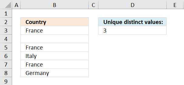
This example demonstrates how to count unique distinct values ignoring blank cells. The UNIQUE function returns 0 (zero) for blank values but the TOCOL function ignores blank values.
Excel 365 formula in cell D3:
Explaining the formula in cell D3
Step 1 - List unique distinct values
The UNIQUE function returns a unique or unique distinct list.
Function syntax: UNIQUE(array,[by_col],[exactly_once])
UNIQUE(B3:B8)
returns {"France";"Germany";0;"Italy"}
Step 2 - Ignore blank cells
The TOCOL function rearranges values in 2D cell ranges to a single column.
Function syntax: TOCOL(array, [ignore], [scan_by_col])
TOCOL(UNIQUE(B3:B8),1)
returns {"France";"Germany";"Italy"}.
Step 3 - Count nonempty values in the array
The COUNTA function counts the non-empty or non-blank cells in a cell range.
Function syntax: COUNTA(value1, [value2], ...)
COUNTA(UNIQUE(B3:B8))
returns 3.
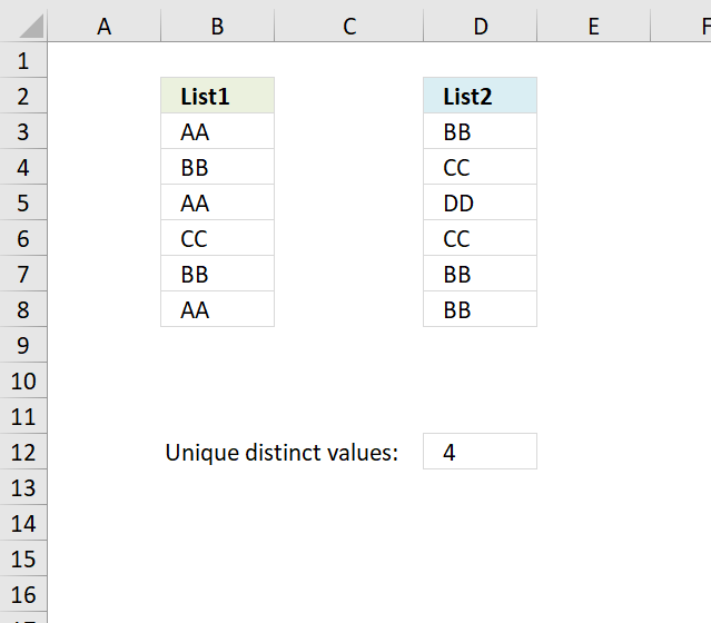
3 Count unique distinct values in multiple nonadjacent cell ranges - Excel 365

This example demonstrates an Excel 365 that counts unique distinct values in multiple cell ranges, the TOCOL function lets you add multiple cell ranges.
The cell ranges don't need to be the same size or adjacent or for that matter on the same worksheet, you can also reference a cell range containing multiple columns.
Excel 365 dynamic array formula in cell D14:
Explaining formula
Step 1 - Join cell ranges
The TOCOL function rearranges values in 2D cell ranges to a single column.
Function syntax: TOCOL(array, [ignore], [scan_by_col])
TOCOL((B3:B8,D3:D7))
returns {"AA"; "BB"; ... ; "BB"}.
Step 2 - List unique distinct values
The UNIQUE function returns a unique or unique distinct list.
Function syntax: UNIQUE(array,[by_col],[exactly_once])
UNIQUE(TOCOL((B3:B8,D3:D7)))
returns {"AA";"BB";"CC";"DD"}.
Step 3 - Count nonempty values
The COUNTA function counts the non-empty or non-blank cells in a cell range.
Function syntax: COUNTA(value1, [value2], ...)
COUNTA(UNIQUE(TOCOL((B3:B8,D3:D7)))) returns 4
4. Count unique distinct values
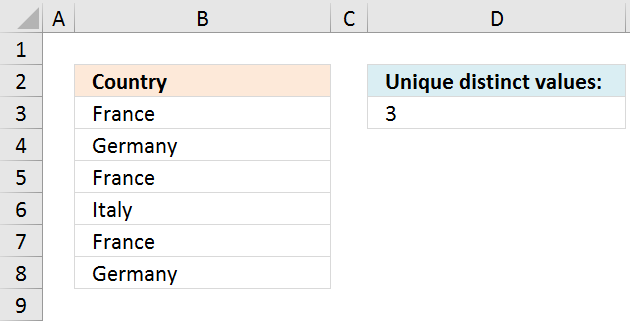
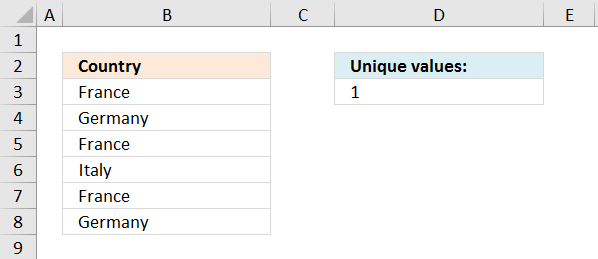
The total number of unique distinct values are calculated in cell D3. The formula is not case sensitive, in other words, value FRANCE is the same as france.
Formula in cell E3:
Recommended article:
Recommended articles
This article demonstrates how to construct a formula that counts unique distinct values based on a condition. The image above […]
Watch a video where I explain the formula
The following formula is an array formula although slightly smaller than the regular formula above, however, you need to enter it as an array formula.
Keep in mind that if you have a blank in your cell range the formulas above won't work, read this: Count unique distinct values in a cell range with blanks
4.1 How the formula works
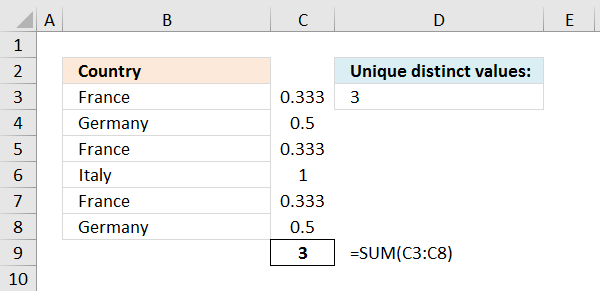
=SUMPRODUCT(1/COUNTIF($B$3:$B$8, $B$3:$B$8))
Step 1 - Count each value
COUNTIF($B$3:$B$8, $B$3:$B$8)
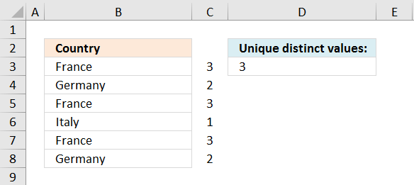
returns an array shown in column C in the picture below.
Recommended articles

Counts the number of cells that meet a specific condition.
Step 2 - Divide 1 with array
1/COUNTIF($B$3:$B$8, $B$3:$B$8)
returns an array shown in column C on the picture below.
Step 3 - Sum values
SUMPRODUCT(1/COUNTIF($B$3:$B$8, $B$3:$B$8))
returns 3.
The array of numbers is located in cell range C3:C8
Recommended articles
What is the SUM function? The SUM function in Excel allows you to add numerical values and returning a total, […]
5. Count unique distinct values in a cell range with blanks
Array formula in cell D3:
Watch a youtube video where I explain the formula
Alternative array formula
Recommended article
Recommended articles
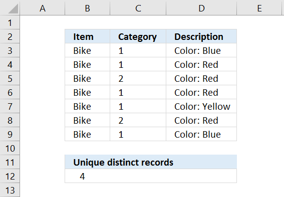
Table of Contents Count unique distinct records Count records with possible blank rows in data set How to count blank […]
How to create an array formula
- Copy (Ctrl + c) and paste (Ctrl + v) array formula into formula bar.
- Press and hold Ctrl + Shift.
- Press Enter once.
- Release all keys.
Recommended articles

Array formulas allows you to do advanced calculations not possible with regular formulas.
Get excel example file
count-unique-distinct-values-in-a-column.xls
(Excel 97-2003 Workbook *.xls)
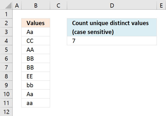
6. Count unique distinct values (case sensitive)
Array formula in cell D4:
Watch a video where I explain the formula
Recommended article
Extract unique distinct values (case sensitive) [Formula]
Recommended articles

First, let me explain the difference between unique values and unique distinct values, it is important you know the difference […]
How to enter an array formula
- Select cell C2
- Press with left mouse button on in formula bar
- Paste above array formula
- Press and hold Ctrl + Shift
- Press Enter
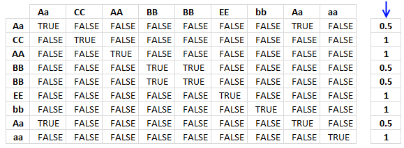
6.1 Explaining array formula in cell D4
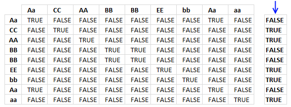
Step 1 - Compare values against each other using the EXACT function
EXACT($B$3:$B$11, TRANSPOSE($B$3:$B$11))
eturns the following boolean array, shown in picture below. Boolean values are TRUE or FALSE.
I have added the original values horizontally and vertically, they are also bolded.
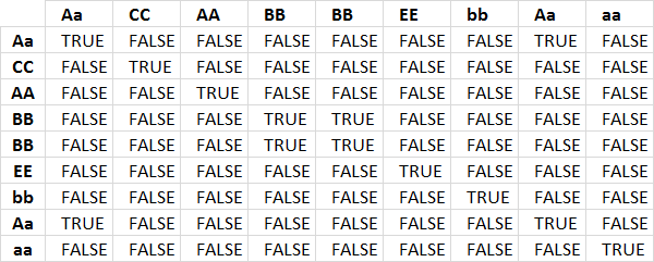
The first column shows that value Aa exists twice because there are two TRUE in the first row.
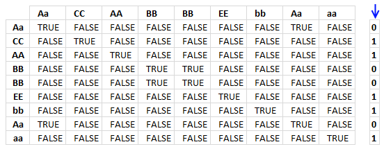
Step 2 - Add values row-wise
The MMULT function allows you to add numbers for each row. To be able to do that I need to convert the boolean values to integers, in this case 0 or 1.
The MMULT function needs two arguments, the second argument must be an array of 1's with the same number of rows as the array in the first argument.
MMULT(EXACT($B$3:$B$11, TRANSPOSE($B$3:$B$11))*1, ROW($B$3:$B$11)^0)
returns an array displayed in the column to the right in the image below.
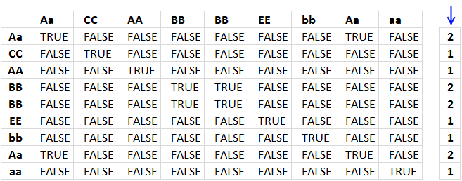
Step 3 - Divide 1 with array
1/MMULT(EXACT($B$3:$B$11, TRANSPOSE($B$3:$B$11))*1, ROW($B$3:$B$11)^0)
returns an array displayed in the image below under the blue arrow.
Step 4 - Sum values
=SUM(--(MMULT(EXACT($B$3:$B$11, TRANSPOSE($B$3:$B$11))*1, ROW($B$3:$B$11)^0)=1))
becomes
=SUM({0.5; 1; 1; 0.5; 0.5; 1; 1; 0.5; 1})
and returns 7 in cell D4.
Get excel *.xlsx file
Count unique distinct values case sensitive.xlsx
7. Count unique distinct values in two columns
Formula in C12:
How to create an array formula
- Double press with left mouse button on cell C12
- Paste above formula
- Press and hold Ctrl + Shift
- Press Enter
Explaining formula in cell C12
Step 1 - Count values in cell range B3:B8
The COUNTIF function counts values equal to a condition or criteria.
COUNTIF($B$3:$B$8, $B$3:$B$8)
returns {3;2;3;1;2;3}
Step 2 - Divide 1 with array
1/COUNTIF($B$3:$B$8, $B$3:$B$8)
returns {0.333333333333333;... ;0.333333333333333}
Step 3 - Sum values
The SUM function simply adds the numbers and returns the total.
SUM(1/COUNTIF($B$3:$B$8, $B$3:$B$8))
returns 3.
Step 4 - Which values exist in cell range $D$3:$D$8
COUNTIF($B$3:$B$8, $D$3:$D$8)=0
returns {FALSE; FALSE;...; FALSE}
Step 5 - Convert TRUE to corresponding number
The IF function uses a logical expression (argument1) to determine which value to return (TRUE - argument2 , FALSE - argument3)
IF(COUNTIF($B$3:$B$8, $D$3:$D$8)=0, 1/COUNTIF($D$3:$D$8, $D$3:$D$8), 0)
returns {0;0;1;0;0;0}.
Step 6 - Sum array
SUM(IF(COUNTIF($B$3:$B$8, $D$3:$D$8)=0, 1/COUNTIF($D$3:$D$8, $D$3:$D$8), 0))
becomes SUM({0;0;1;0;0;0}) and returns 1.
Step 7 - Add numbers
SUM(1/COUNTIF($B$3:$B$8, $B$3:$B$8))+SUM(IF(COUNTIF($B$3:$B$8, $D$3:$D$8)=0, 1/COUNTIF($D$3:$D$8, $D$3:$D$8), 0))
becomes 3+1 and returns 4 in cell D12.
Get Excel *.xlsx file
Count unique distinct values in two columns.xlsx
8. Count unique distinct months
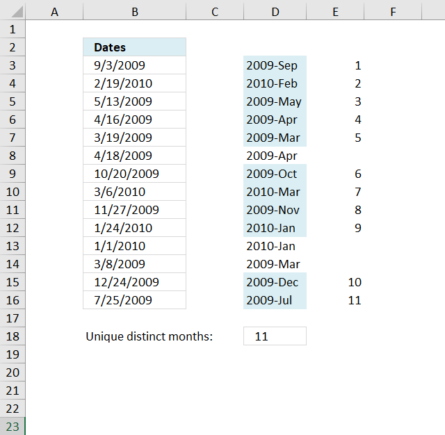
The formula in cell D18 counts unique distinct months in cell range B3:B16.
Formula in D18:
Explaining formula in cell D18
Step 1 - Convert dates
The DATE function changes each date to the first in the given month and year.
DATE(YEAR($B$3:$B$16), MONTH($B$3:$B$16), 1)
returns {40057; 40210; ... ; 39995}
Step 2 - Count frequency of each number
The FREQUENCY function returns an array of numbers representing how many times the number occurs in the list.
FREQUENCY(DATE(YEAR($B$3:$B$16),MONTH($B$3:$B$16),1),DATE(YEAR($B$3:$B$16),MONTH($B$3:$B$16),1))
returns {1;1;1;...;0}.
Step 3 - Check if value is larger than 0 (zero)
We know a value is unique distinct if it is larger than 0 (zero).
(FREQUENCY(DATE(YEAR($B$3:$B$16),MONTH($B$3:$B$16),1),DATE(YEAR($B$3:$B$16),MONTH($B$3:$B$16),1))>0
returns {TRUE; TRUE; ... ; FALSE}
Step 4 - Convert boolean values
We must first convert the boolean values in order to sum the values, multiply with 1 to create their numerical equivalents.
(FREQUENCY(DATE(YEAR($B$3:$B$16), MONTH($B$3:$B$16), 1), DATE(YEAR($B$3:$B$16), MONTH($B$3:$B$16), 1))>0)*1
returns {1;1;... ;0}.
Step 5 - Sum values
Use the SUMPRODUCT function to add the numbers and return a total.
SUMPRODUCT((FREQUENCY(DATE(YEAR($B$3:$B$16),MONTH($B$3:$B$16),1),DATE(YEAR($B$3:$B$16),MONTH($B$3:$B$16),1))>0)*1)
becomes SUMPRODUCT({1;1;1;1;1;0;1;1;1;1;0;0;1;1;0}) and returns 11 in cell D18.
Get Excel *.xlsx
Count unique distinct months.xlsx
9. Count digits and ignore duplicates

I have a question that I can’t seem to find an answer to:
I want to make a full count of digits 0 to 9 while ignoring duplicates in any line
B C D E
5 5 5 5
8 6 7 4
6 2 8 7
7 7 1 6
5 6 6 2For example, with the digits shown above, my results for the count will be:
0=0; 1=1; 2=2; 3=0; 4=1; 5=5; 6=4; 7=3; 8=2; 9=0
The formula below does not work for the “5” count since it counts all the occurrences:
=COUNTIF($B$1:$E$5,5)
Answer:
I can't achieve the desired result for number 5. I calculated any line as "in any row" and "in any column". I guess the desired result for number 5 is a typo.
Array formula in cell B9:
Copy cell B9 and paste down as far as needed.
Array formula in cell C9:
Copy cell C9 and paste down as far as needed.
How the formula works in cell B9
Step 1 - Find digit in array
A9=$B$1:$E$5
returns {FALSE, FALSE, ... , FALSE}
Step 2 - Convert boolean array to row numbers
IF(A9=$B$1:$E$5, ROW($B$1:$E$5)-MIN(ROW($B$1:$E$5))+1, "")
returns {"", "", ... , ""}
Step 3 - Count row numbers
FREQUENCY(data_array, bins_array)
Calculates how often values occur within a range of values and then returns a vertical array of numbers having one more element than Bins_array.
FREQUENCY(IF(A9=$B$1:$E$5, ROW($B$1:$E$5)-MIN(ROW($B$1:$E$5))+1, ""), ROW($1:$5))
returns {0; 0; 0; 0; 0}
Step 4 - Count numbers larger than zero
=SUM(IF(FREQUENCY(IF(A9=$B$1:$E$5, ROW($B$1:$E$5)-MIN(ROW($B$1:$E$5))+1, ""), ROW($1:$5))>0, 1, 0))
becomes SUM({0; 0; 0; 0; 0}) and returns 0 (zero).
10. Count unique distinct values in a large dataset - UDF

This article describes how to count unique distinct values in list. What is a unique distinct list? Merge all duplicates to one distinct value and you have created a unique distinct list.
Formulas are sometimes too slow if you work with a lot of data, this article demonstrates a user defined function you can use, however, I highly recommend using a pivot table for this task:
Count unique distinct values using a pivot table
Formula in cell H2:
Excel user defined function
Public Function CountUniqueValues(rng As Variant) As Variant

Dim Test As New Collection
Dim Value As Variant

rng = rng.Value

On Error Resume Next
For Each Value In rng

If Len(Value) > 0 Then Test.Add Value, CStr(Value)

Next Value
On Error GoTo 0

CountUniqueValues = Test.Count

End Function
How to add the user defined function to your workbook
1. Press Alt-F11 to open the visual basic editor
2. Press with left mouse button on Module on the Insert menu
3. Copy and paste the above user defined function
4. Exit visual basic editor
5. Select a sheet
6. Select a cell range
7. Type =CountUniqueValues(A1:F3000) into formula bar and press ENTER
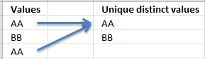
11. Count unique values in a column
Unique values are values that exist only once, see picture below.
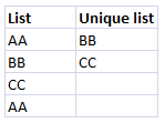
AA has a duplicate and is not unique. BB and CC have no duplicates and are unique.
Formula in D3:
There is only one unique value in the list (Italy), all other values have duplicates.
Watch a video where I explain the formula
Explaining formula in cell C3
Step 1 - Count all values
The COUNTIF function counts how many values in a cell range that match a condition. In this case, the second argument has multiple values and this makes the COUNTIF function return an array of values.
COUNTIF($B$3:$B$8,$B$3:$B$8)
returns an array displayed in cell range C3:C8 in the image below.
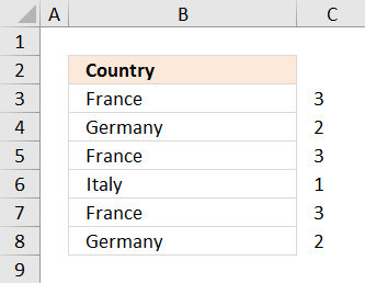
This array tells us that the value France exists three times in cell range B3:B8. Germany exists twice and Italy is a unique value meaning there is only one instance of Italy in cell range B3:B8.
Learn more about the COUNTIF function here:
Recommended articles
Counts the number of cells that meet a specific condition.
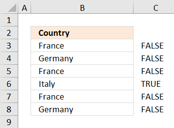
Step 2 - Check each value is equal to 1
COUNTIF($B$3:$B$8,$B$3:$B$8)=1
returns the array displayed in cell range C3:C8
Step 3 - Convert boolean values to integers
To be able to sum the boolean values I need to convert them to their equivalent 0 and 1. TRUE is 1 and FALSE is 0.
--(COUNTIF($B$3:$B$8,$B$3:$B$8)=1)
returns the array displayed in cell range C3:C8
Step 4 - Sum values
=SUMPRODUCT(--(COUNTIF($B$3:$B$8,$B$3:$B$8)=1))
returns 1 in cell D3.
Get excel example file
count-unique-distinct-values-in-a-column.xls
(Excel 97-2003 Workbook *.xls)
Recommended blog posts:
Count unique distinct records in Excel
12. Count unique values (case sensitive)
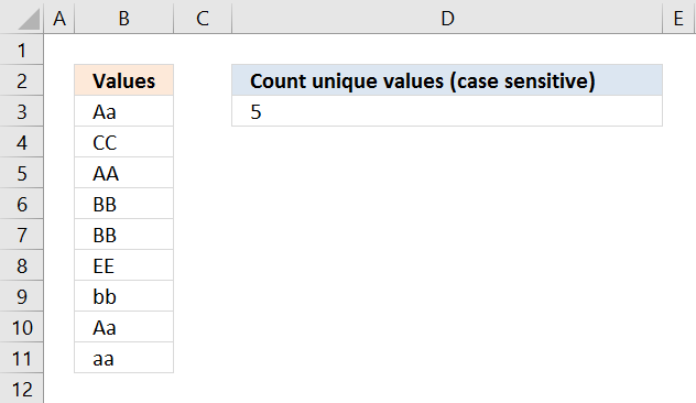
The picture below shows values in column B, the formula in cell D3 counts 5 unique values in column B.
They are CC, AA, EE, bb and aa. They only exist once in column B.
Aa and BB have duplicates and are not unique.
Array formula in cell D3:
Watch a video where I explain the formula
12.1 Explaining array formula in cell D3
Step 1 - Compare values against each other using the EXACT function
EXACT($B$3:$B$11, TRANSPOSE($B$3:$B$11))
returns the following boolean array, shown in picture below. Boolean values are TRUE or FALSE.
I have added the original values horizontally and vertically, they are also bolded.
The first column shows that value Aa exists twice because there are two TRUE in the first row.
Step 2 - Add values row-wise
The MMULT function allows you to add numbers for each row. To be able to do that I need to convert the boolean values to integers, in this case 0 or 1.
The MMULT function needs two arguments, the second argument must be an array of 1's with the same number of rows as the array in the first argument.
MMULT(EXACT($B$3:$B$11, TRANSPOSE($B$3:$B$11))*1, ROW($B$3:$B$11)^0)
returns an array shown in the column to the right below the blue arrow.
Step 3 - Check if values in array are equal to 1
MMULT(EXACT($B$3:$B$11, TRANSPOSE($B$3:$B$11))*1, ROW($B$3:$B$11)^0)=1
returns an array shown in the column to the right below the blue arrow.
Step 4 - Convert boolean values to integers
The SUM function can't add boolean values, to be able to do that I need to convert boolean values to integers.
--(MMULT(EXACT($B$3:$B$11, TRANSPOSE($B$3:$B$11))*1, ROW($B$3:$B$11)^0)=1)
returns an array shown in the column to the right below the blue arrow.
Step 5 - Sum values
=SUM(--(MMULT(EXACT($B$3:$B$11, TRANSPOSE($B$3:$B$11))*1, ROW($B$3:$B$11)^0)=1))
becomes SUM({0;1;1;0;0;1;1;0;1}) and returns 5 in cell D3.
Get excel *.xlsx file
Count unique values case sensitive.xlsx
13. Count unique distinct values within same week, month or year
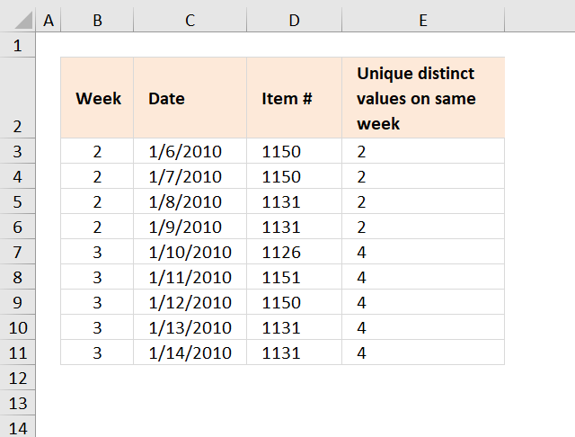
The array formula in cell E3 counts unique distinct items for all dates within the same week. Example, week 2 has two unique distinct items: 1150 and 1131.
Unique distinct values are all values but duplicates are merged into one value.
Formula in B3:
Array formula in E3:
How to create an array formula
- Copy (Ctrl + c) and paste (Ctrl + v) array formula into formula bar.
- Press and hold Ctrl + Shift.
- Press Enter once.
- Release all keys.
Copy cell E3 and paste it down as far as needed.
Item is named range pointing to cell range D3:D11.
Explaining array formula in cell E3
=SUM(--((FREQUENCY(IF(YEAR(C3)&"-"&B3=YEAR($C$3:$C$11)&"-"&$B$3:$B$11, Item, ""), Item))>0))
Step 1 - Filter records in date range
IF(YEAR(C3)&"-"&B3=YEAR($C$3:$C$11)&"-"&$B$3:$B$11, Item, "")
returns {1150;1150;1131;1131;"";"";"";"";""}
Step 2 - Calculate frequency
FREQUENCY(IF(YEAR(C3)&"-"&B3=YEAR($C$3:$C$11)&"-"&$B$3:$B$11, Item, ""), Item))
returns {2;0;2;0;0;0;0;0;0;0}
Step 3 - Count and sum values larger than 0 (zero)
SUM(--((FREQUENCY(IF(YEAR(C3)&"-"&B3=YEAR($C$3:$C$11)&"-"&$B$3:$B$11, Item, ""), Item))>0))
becomes =SUM({1;0;1;0;0;0;0;0;0;0}) and returns 2 in cell E3.
Get Excel *.xlsx file
Count-unique-occurences-within-same-week-month-year.xlsx
Count unique distinct values within same month

Array formula in E16:
How to create an array formula
- Copy (Ctrl + c) and paste (Ctrl + v) array formula into formula bar.
- Press and hold Ctrl + Shift.
- Press Enter once.
- Release all keys.
Copy cell E16 and paste it down as far as needed.
Count unique distinct values within same year

Array formula in E29:
How to create an array formula
- Copy (Ctrl + c) and paste (Ctrl + v) array formula into formula bar.
- Press and hold Ctrl + Shift.
- Press Enter once.
- Release all keys.
Copy cell E29 and paste it down as far as needed.
Get excel sample file
Count-unique-occurences-within-same-week-month-year.xls
14. Introduction
What are unique distinct values?
Unique distinct values are all values except that duplicates are merged into one value, in other words, duplicates are removed.
Is a Pivot Table easier?
Yes, in most cases. I highly recommend you use a pivot table if you own Excel 2013 or a later version.
A pivot table is easier to work with and much faster if you have lots of data:
Count unique distinct values [Pivot Table]
The downside is that you need to manually refresh the pivot table if the source data range changes. You also need to learn how to create and operate Pivot Tables before you can count unique distinct values, however, it is worth it.
When to use formulas in these particular cases?
An array formula is great for an interactive dashboard or dynamic data meaning data changes often, like once a week or perhaps once a month.
My source data range changes often in size, how do I create the formulas more dynamic?
If you use an Excel defined Table or a dynamic named range you can quickly change the data range without editing the cell references in the array formula.
15. How to count unique distinct items based on a condition and a date condition - Excel 365?

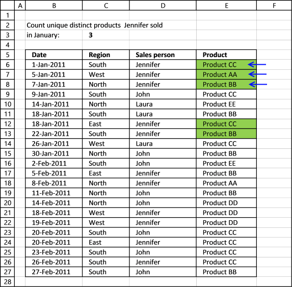
This example shows how to count unique distinct products based on a given salesperson and a given month. Cell range B6:B27 contains dates, C6:C27 contains regions, however, they are not used in this particular example right now. Cell range D6:D27 contains salespersons, E6:E27 contains products.
The date condition is January and the salesperson condition is Jennifer. The formula extracts products from E6:E27 based on these criteria and then returns the count.
Excel 365 dynamic formula in cell C3:
An Excel dynamic array formula is entered as a regular formula, however, it spills values below the cell if needed. This example returns a single value so no need for spilling.
The image above shows products that match the criteria with a different cell background, Product AA and Product BB have duplicates so there are only three unique distinct products. The formula in cell C3 contains the formula and it returns number 3.
15.1 Explaining formula in cell C3
Step 1 - Find dates in January
The MONTH function extracts the month as a number from an Excel date.
Function syntax: MONTH(serial_number)
MONTH(B6:B27)=1
returns {TRUE; TRUE; TRUE; ... ; FALSE}
Step 2 - Find salesperson Jennifer
The equal sing is a logical operator that lets you compare value to value, it returns boolean value TRUE if the match and FALSE if not.
D6:D27="Jennifer"
returns {TRUE; TRUE; TRUE;... ; FALSE}
Step 3 - Which rows have both conditions met
The asterisk lets you multiply boolean values meaning applying AND logic between values on the same row. The parentheses let you control the order of operation which is very important.
(MONTH(B6:B27)=1)*(D6:D27="Jennifer")
returns {1; 1; 1; ... ; 0}
Step 4 - Filter products based on criteria
The FILTER function extracts values/rows based on a condition or criteria.
Function syntax: FILTER(array, include, [if_empty])
FILTER(E6:E27,(MONTH(B6:B27)=1)*(D6:D27="Jennifer"))
returns {"Product CC"; "Product AA"; "Product BB"; "Product CC"; "Product BB"}
Step 5 - Extract unique products
The UNIQUE function returns a unique or unique distinct list.
Function syntax: UNIQUE(array,[by_col],[exactly_once])
UNIQUE(FILTER(E6:E27,(MONTH(B6:B27)=1)*(D6:D27="Jennifer")))
returns {"Product CC"; "Product AA"; "Product BB"}
Step 6 - Count rows in array
The ROWS function calculate the number of rows in a cell range.
Function syntax: ROWS(array)
ROWS(UNIQUE(FILTER(E6:E27,(MONTH(B6:B27)=1)*(D6:D27="Jennifer"))))
becomes
ROWS({"Product CC"; "Product AA"; "Product BB"})
and returns 3.
16. How to count unique distinct items based on two conditions and a date condition - Excel 365?

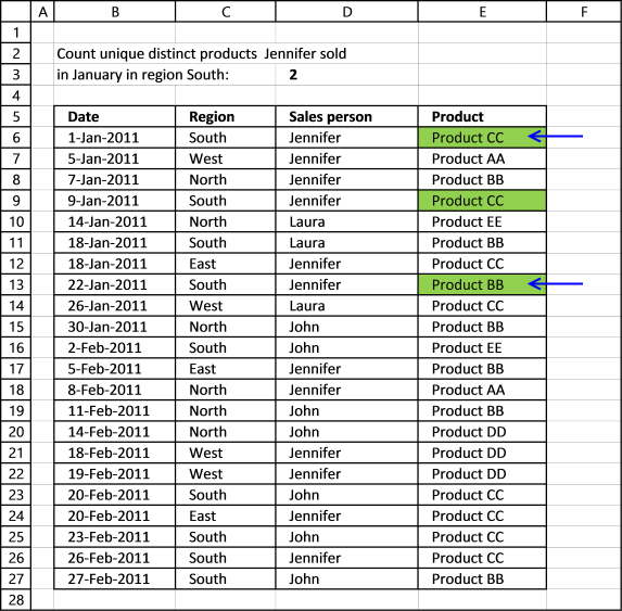
This example demonstrates a formula that counts unique distinct products based on a given salesperson, a given month, and a given region. Cell range B6:B27 contains dates, C6:C27 contains regions, D6:D27 contains salespersons, and E6:E27 contains products.
The date condition is January, the salesperson condition is Jennifer, and the Region is South. The formula extracts products from E6:E27 based on these criteria and then returns the count.
Excel 365 dynamic formula in cell C3:
An Excel dynamic array formula is entered as a regular formula, however, it spills values below the cell if needed. This example returns a single value so no need for spilling.
The image above shows highlighted products that match the criteria , Product CC has a duplicate so there are only two unique distinct products. The formula in cell C3 contains the formula and it returns number 2.
16.1 Explaining formula in cell C3
Step 1 - Find dates in January
The MONTH function extracts the month as a number from an Excel date.
Function syntax: MONTH(serial_number)
MONTH(B6:B27)=1
returns {TRUE; TRUE; TRUE; ... ; FALSE}
Step 2 - Find salesperson Jennifer
The equal sing is a logical operator that lets you compare value to value, it returns boolean value TRUE if the match and FALSE if not.
D6:D27="Jennifer"
becomes
{"Jennifer"; "Jennifer"; "Jennifer"; ... ; "John"}="Jennifer"
and returns
{TRUE; TRUE; TRUE; ... ; FALSE}
Step 3 - Find region south
C6:C27="South"
returns {TRUE; FALSE; FALSE; ... ; TRUE}
Step 4 - Which rows have all three conditions met
The asterisk lets you multiply boolean values meaning applying AND logic between values on the same row. The parentheses let you control the order of operation which is very important.
(MONTH(B6:B27)=1)*(D6:D27="Jennifer")*(C6:C27="South")
returns {1; 0; 0; ... ; 0}
Step 5 - Filter products based on criteria
The FILTER function extracts values/rows based on a condition or criteria.
Function syntax: FILTER(array, include, [if_empty])
FILTER(E6:E27,(MONTH(B6:B27)=1)*(D6:D27="Jennifer")*(C6:C27="South"))
returns {"Product CC"; "Product CC"; "Product BB"}
Step 6 - Extract unique products
The UNIQUE function returns a unique or unique distinct list.
Function syntax: UNIQUE(array,[by_col],[exactly_once])
UNIQUE(FILTER(E6:E27,(MONTH(B6:B27)=1)*(D6:D27="Jennifer")*(C6:C27="South")))
returns {"Product CC";"Product BB"}
Step 7 - Count rows in array
The ROWS function calculate the number of rows in a cell range.
Function syntax: ROWS(array)
ROWS(UNIQUE(FILTER(E6:E27,(MONTH(B6:B27)=1)*(D6:D27="Jennifer")*(C6:C27="South"))))
returns 2.
17. How many unique distinct products were sold in region south or in January?

This Excel 365 formula in cell C3 counts the number of unique distinct products in cell range E6:E27 if the corresponding cells on the same row in C6:C27 equals "South" or dates in B6:B27 is in January.
This example is different than the examples above, this example uses OR logic whereas the examples above uses AND logic.
Excel 365 dynamic formula in cell C3:
This Excel 365 formula is entered as a regular formula, column F in the image above shows the unique distinct count and if an item is a duplicate beginning from top to bottom.
17.1 Explaining formula in cell C3
Step 1 - Find dates in January
The MONTH function extracts the month as a number from an Excel date.
Function syntax: MONTH(serial_number)
MONTH(B6:B27)=1
returns {TRUE; TRUE; TRUE; ... ; FALSE}
Step 2 - Find region South
The equal sing is a logical operator that lets you compare value to value, it returns boolean value TRUE if the match and FALSE if not.
returns {TRUE; FALSE; FALSE; ... ; TRUE}
Step 3 - Which rows have at least on of the conditions met
The plus sign + lets you add boolean values meaning applying OR logic between values on the same row. The parentheses let you control the order of operation which is very important.
(MONTH(B6:B27)=1)+(C6:C27="South")
returns {2; 1; 1; ... ; 1}
Step 4 - Filter products based on criteria
The FILTER function extracts values/rows based on a condition or criteria.
Function syntax: FILTER(array, include, [if_empty])
FILTER(E6:E27,(MONTH(B6:B27)=1)+(C6:C27="South"))
returns {"Product CC"; "Product AA"; "Product BB"; ... ; "Product BB"}
Step 5 - Extract unique products
The UNIQUE function returns a unique or unique distinct list.
Function syntax: UNIQUE(array,[by_col],[exactly_once])
UNIQUE(FILTER(E6:E27,(MONTH(B6:B27)=1)+(C6:C27="South")))
returns {"Product CC"; "Product AA"; "Product BB"; "Product EE"}
Step 6 - Count rows in array
The ROWS function calculate the number of rows in a cell range.
Function syntax: ROWS(array)
ROWS(UNIQUE(FILTER(E6:E27,(MONTH(B6:B27)=1)+(C6:C27="South"))))
returns 4.
18. How to count unique distinct items based on a condition and a date condition?
This example works with Excel versions prior to Excel 365, it describes a formula that counts the unique distinct products Jennifer sold in January? In other words, it extracts a unique distinct list based on three conditions.
Cell range B6:B27 contains dates, C6:C27 contains regions, D6:D26 contains salespersons, and E6:E27 contains items.
Array formula in C3:
This is an array formula and is entered differently than a regular formula. To enter an array follow these steps:
- Double press with left mouse button on the destination cell, a prompt appears.
- Type or copy/paste the formula.
- Press and hold CTRL and SHIFT keys simultaneously.
- Press Enter once.
- Release all keys.
A beginning and ending curly bracket appears like this:
{=SUM(IF(("Jennifer"=$D$6:$D$27)*($B$6:$B$27<=DATE(2011, 1, 31)), 1/COUNTIFS($D$6:$D$27, "Jennifer", $E$6:$E$27, $E$6:$E$27, $B$6:$B$27, "<="&DATE(2011, 1, 31))), 0))}
Don't enter the curly brackets yourself, they appear automatically if you followed the above steps.
18.1.1 Watch this video where I explain how the above formula works
This calculation is also possible using a pivot table, you simply add more criteria: Count unique distinct values [Pivot Table]
18.1.2 Explaining formula in cell C3
Step 1 - Find values meeting first condition
The equal sign compares the condition (Jennifer) to all cell values in $D$6:$D$27 and returns an array containing TRUE or FALSE (boolean values).
("Jennifer"=$D$6:$D$27)
returns {TRUE; TRUE; TRUE; ... ; FALSE}
Step 2 - Find values meeting the second condition
The less than < and equal sign together lets you compare Date 1/31/2011 with dates in $B$6:$B$27, it returns TRUE if the date is earlier than or equal to 1/31/2011.
($B$6:$B$27<=DATE(2011, 1, 31))
returns {TRUE; TRUE; TRUE; ... ; FALSE}
Step 3 - Calculate the number of records that contain condition 1 and 2 and any products
The COUNTIFS function calculates the number of cells across multiple ranges that equals all given conditions. There is a criteria range and a condition forming a pair.
| Pair | Criteria range | Criteria |
| 1 | $D$6:$D$27 | "Jennifer" |
| 2 | $E$6:$E$27 | $E$6:$E$27 |
| 3 | $B$6:$B$27 | "<="&DATE(2011, 1, 31) |
1/COUNTIFS($D$6:$D$27, "Jennifer", $E$6:$E$27, $E$6:$E$27, $B$6:$B$27, "<="&DATE(2011, 1, 31)))
returns {0.5; 1; 0.5; ... ; 0.5}
Step 4 - If condition 1 and 2 are TRUE then return numbers from step 3
The IF function has three arguments, the first one must be a logical expression. If the expression evaluates to TRUE then one thing happens (argument 2) and if FALSE another thing happens (argument 3).
IF(("Jennifer"=$D$6:$D$27)*($B$6:$B$27<=DATE(2011, 1, 31)), 1/COUNTIFS($D$6:$D$27, "Jennifer", $E$6:$E$27, $E$6:$E$27, $B$6:$B$27, "<="&DATE(2011, 1, 31))), 0)
You get the numerical equivalents if you add or multiply arrays, the numerical equivalent of TRUE is 1 and FALSE is 0 (zero),
returns {0.5; 1; ... ; 0}
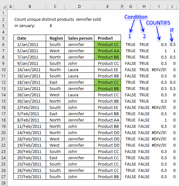
The image above shows the results of each step.
- Step 1 - Column G
- Step 2 - Column H
- Step 3 - Column I
- Step 4 - Column J
Step 5 - Sum numbers in array
SUM(IF("Jennifer"=$D$5:$D$26, 1/(COUNTIFS($D$5:$D$26, "Jennifer", $E$5:$E$26, $E$5:$E$26)), 0))
returns 3 in cell C3. There are three unique distinct products based on two conditions.
19. How many unique distinct products did Jennifer sell in January and in region South?
How many unique distinct products did Jennifer sell in January and in region South?
Array formula in D3:
20. How many unique distinct products was sold in the south or in January?
How many unique distinct products was sold in the south or in January?
Array formula:
21. Count unique distinct records
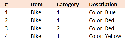
The image above shows a table with 3 columns containing random data. It is quite complicated trying to manually count unique distinct records from this table but Excel can do that for us. A record is an entire row in the table above.
Example, Row 3 has a duplicate in row 9. Row 4 has a duplicate in row 6. Row 5 has a duplicate in row 8. Row 7 is unique meaning there is only one instance of that record in the table. It is also possible to highlight unique distinct records using conditional formatting.
Formula in cell B12:
21.1.1 Watch a video where I explain the formula
We can verify the count above in cell B12 by extracting all unique distinct records from the above table. I am using a formula from this blog article:
Filter unique distinct row records
21.1.2 Explaining formula in cell B12
Step 1 - Count each record in data set
COUNTIFS(C3:C9,C3:C9,D3:D9,D3:D9,E3:E9,E3:E9) counts the number of times all criteria match on each row
Example,
The first record is Bike, 1, Color: Blue. The only rows where these criteria match is the first one and last. So the first number in the returning array is 2.
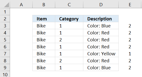
I have entered =COUNTIFS(C3:C9,C3:C9,D3:D9,D3:D9,E3:E9,E3:E9) in column E.
COUNTIFS(C3:C9,C3:C9,D3:D9,D3:D9,E3:E9,E3:E9) returns {2;2;2;2;1;2;2}
Step 2 - Divide 1 with array
Why divide 1 with array? If there are two instances of a value the sum returns 1 (0.5 + 0.5 = 1), three instances returns 1 (1/3 + 1/3 + 1/3 = 1) and so on. This lets you count all instances of a value as one.
1/COUNTIFS(C3:C9,C3:C9,D3:D9,D3:D9,E3:E9,E3:E9)
becomes
1/{2;2;2;2;1;2;2}
and returns {0.5;0.5;0.5;0.5;1;0.5;0.5}
Step 3 - Sum values in array
The SUMPRODUCT function lets you sum values, in this case, without entering it as an array formula.
SUMPRODUCT(1/COUNTIFS(C3:C9,C3:C9,D3:D9,D3:D9,E3:E9,E3:E9))
becomes
SUMPRODUCT({0.5;0.5;0.5;0.5;1;0.5;0.5})
and returns 4 in cell range B12
22. Count records with possible blank rows in data set
![]()
Array formula in cell A28:
To enter an array formula, type the formula in a cell then press and hold CTRL + SHIFT simultaneously, now press Enter once. Release all keys.
The formula bar now shows the formula with a beginning and ending curly bracket telling you that you entered the formula successfully. Don't enter the curly brackets yourself.
23. How to count blank rows/records
![]()
Formula in B28:
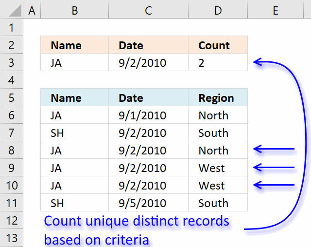
24. Count unique distinct records with a date and column criteria
re: Count records between two dates and a criterion
based on the example, i was looking for 1 date and 1 criterion. i slightly modify the formula to
=SUMPRODUCT(--($B$1:$B$9=$E$2), --($A$1:$A$9=$E$3)) + ENTER
[assuming E2 = 9-2-2010]
the result would be 1 (one 'JA' found on 9-2-2010 date)
but this is summation of records found on 1 date with 1 criterion. It will not work if there is *multiple* 'JA' criterion exist on the same date because SUMPRODUCT summed up the records found.
I'm curious to know...
1) What if I want to know the UNIQUE DISTINCT records found on 1 date with 1 criterion?
2) Working on >100k rows of data, this formula literally slows down Excel (heavy calculation and recalculations). Is there an alternative to speed it up? UDF? array formula?
thanks!
Answer:
Array formula in cell D3:
How to create an array formula
- Copy (Ctrl + c) and paste (Ctrl + v) array formula into formula bar.
- Press and hold Ctrl + Shift.
- Press Enter once.
- Release all keys.
How the array formula in cell D3 works
Step 1 - Count records
The COUNTIFS function calculates the number of cells across multiple ranges that equals all given conditions.
COUNTIFS($B$6:$B$11, $B$6:$B$11, $C$6:$C$11, $C$6:$C$11, $D$6:$D$11, $D$6:$D$11)
becomes
COUNTIFS({"JA";"SH";"JA"; "JA";"JA";"SH"}, {"JA";"SH";"JA"; "JA";"JA";"SH"}, {40422;40423; 40423;40423;40423;40426}, {40422;40423; 40423;40423;40423;40426}, {"North";"South";"North"; "West";"West";"South"}, {"North";"South";"North"; "West";"West";"South"})
and returns array {1;1;1;2;2;1}
Step 2 - Filter records using name and date criteria
The IF function returns one value (argument2) if TRUE and another (argument3) if FALSE.
IF(($B$6:$B$11=B3)*($C$6:$C$11=C3), (1/COUNTIFS($B$6:$B$11, $B$6:$B$11, $C$6:$C$11, $C$6:$C$11, $D$6:$D$11, $D$6:$D$11)), 0)
becomes
IF(($B$6:$B$11=B3)*($C$6:$C$11=C3), (1/{1;1;1;2;2;1}), 0)
becomes
IF(({"JA";"SH";"JA";"JA";"JA";"SH"}="JA")*({40422;40423;40423;40423;40423;40426}=40423), (1/{1;1;1;2;2;1}), 0)
becomes
IF(({0;0;1;1;1;0}, (1/{1;1;1;2;2;1}), 0)
becomes
IF(({0;0;1;1;1;0}, {1;1;1;0,5;0,5;1}, 0)
and returns {0;0;1;0,5;0,5;0}
Step 3 - Sum values
The SUM function adds numbers an return the total.
=SUM(IF(($B$6:$B$11=B3)*($C$6:$C$11=C3), (1/COUNTIFS($B$6:$B$11, $B$6:$B$11, $C$6:$C$11, $C$6:$C$11, $D$6:$D$11, $D$6:$D$11)), 0))
becomes
=SUM({0;0;1;0,5;0,5;0}) and returns 2 in cell D3.
25. Count unique distinct values based on a condition

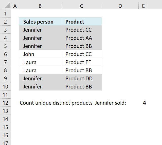
The image above shows a table in columns B and C. Column B contains names and column C contains products. How many unique distinct products did Salesperson Jennifer sell?
The blue arrows show unique distinct products based on salesperson "Jennifer", the total number matches the number in cell E4. The remaining highlighted records are only duplicate values.
Array formula in cell E2:
25.1 How to create an array formula
- Copy (Ctrl + c) and paste (Ctrl + v) array formula into formula bar.
- Press and hold Ctrl + Shift.
- Press Enter once.
- Release all keys.
25.2 Explaining array formula in cell E2
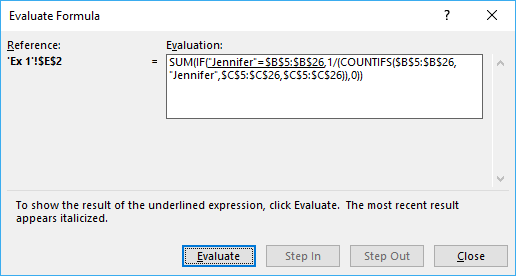
You can follow along as I explain the formula, select cell E2. Go to tab "Formulas" on the ribbon, press with left mouse button on "Evaluate formula" button.
Press with mouse on "Evaluate" button shown in above image to move to next step.
Step 1 - Calculate unique distinct products that Jennifer sold
The COUNTIFS function calculates the number of cells across multiple ranges that equals all given conditions.
COUNTIFS(criteria_range1, criteria1, [criteria_range2, criteria2]…)
1/(COUNTIFS($B$5:$B$26, "Jennifer", $C$5:$C$26, $C$5:$C$26))
returns {0,25; 0,5; 0,333333333333333; ... ; 0,333333333333333}

Step 2 - Filter Jennifers products
The IF function returns one value if the logical test is TRUE and another value if the logical test is FALSE.
IF(logical_test, [value_if_true], [value_if_false])
IF("Jennifer"=$B$5:$B$26, 1/(COUNTIFS($B$5:$B$26, "Jennifer", $C$5:$C$26, $C$5:$C$26)), 0)
returns {0,25; 0,5; 0,333333333333333; ... ; 0}

Step 3 - Sum array
The SUM function allows you to add numbers, the function returns the sum in the cell it is entered in. The SUM function is cleverly designed to ignore text and boolean values, adding only numbers.
SUM(number1, [number2], ...)
SUM(IF("Jennifer"=$B$5:$B$26, 1/(COUNTIFS($B$5:$B$26, "Jennifer", $C$5:$C$26, $C$5:$C$26)), 0))
returns 4 in cell E2.
26. Count unique distinct values based on a condition - Excel 365

This example demonstrates a smaller formula that works only in Excel 365, two out of three functions are Excel 365 functions.
Dynamic array formula in cell F28:
This formula is entered as a regular formula.
26.1 Explaining formula in cell F28
Step 1 - Check which values meet the condition specified in cell C26
The equal sign lets you compare value to value, in this case, value to values. The output is an array of boolean values True or False.
B3:B24=C26
returns {TRUE; TRUE; TRUE; ... ; FALSE}
Step 2 - Filter values
The FILTER function lets you extract values/rows based on a condition or criteria. It is in the Lookup and reference category and is only available to Excel 365 subscribers.
FILTER(C3:C24,B3:B24=C26)
returns {"Product CC"; "Product AA"; "Product BB"; ... ; "Product CC"}.
Step 3 - Extract unique distinct values
The UNIQUE function lets you extract both unique and unique distinct values and also comparing columns to columns or rows to rows.
UNIQUE(FILTER(C3:C24,B3:B24=C26))
returns {"Product CC"; "Product AA"; "Product BB"; "Product DD"}.
Step 4 - Return number of rows in array
The ROWS function returns the number of rows based on a cell range or array.
ROWS(UNIQUE(FILTER(C3:C24,B3:B24=C26)))
returns 4.
27. How to count unique distinct values based on a date

The array formula in cell D3 calculates the number of unique distinct items based on the given date in column B. Unique distinct values are all values but duplicates are merged into one value.
Example, there are five items on date 1/5/2010 in the table above. 1150, 1126, 1131, 1131 and 1126, however there are only three unique distinct items 1150, 1126 and 1131 and that number is what the formula returned in cell D3.
Excel 365 dynamic array formula in cell D3:
Array formula in D3:
To enter an array formula, type the formula in a cell then press and hold CTRL + SHIFT simultaneously, now press Enter once. Release all keys.
The formula bar now shows the formula with a beginning and ending curly bracket telling you that you entered the formula successfully. Don't enter the curly brackets yourself.
Copy cell D3 and paste it down as far as needed.
Explaining formula in cell D3
Step 1 - Calculate alphabetical rank
The COUNTIF function counts values based on a condition or criteria, in this case I use the ampersand to concatenate a less than sign. This will return a number representing the rank in an alphabetically sorted list.
COUNTIF($C$3:$C$11, "<"&$C$3:$C$11)
returns {6;0;2;2;0;6;6;2;2}
Step 2 - Extract numbers based on date
The IF function has three arguments, the first one must be a logical expression. If the expression evaluates to TRUE then one thing happens (argument 2) and if FALSE another thing happens (argument 3).
IF(B3=$B$3:$B$11, COUNTIF($C$3:$C$11, "<"&$C$3:$C$11), "")
returns {6;0;2;2;0;"";"";"";""}.
Step 3 - Cacluate frequency
The FREQUENCY function calculates how often values occur in a range.
FREQUENCY(IF(B3=$B$3:$B$11, COUNTIF($C$3:$C$11, "<"&$C$3:$C$11), ""), (COUNTIF($C$3:$C$11, "<"&$C$3:$C$11))
returns {1;2;2;0;0;0;0;0;0;0}
Step 4 - Is number larger than 0 (zero)?
The value is unique distinct if the corresponding number in the array is larger than 0 (zero).
FREQUENCY(IF(B3=$B$3:$B$11, COUNTIF($C$3:$C$11, "<"&$C$3:$C$11), ""), (COUNTIF($C$3:$C$11, "<"&$C$3:$C$11))>0
returns {TRUE; TRUE; TRUE; FALSE; FALSE; FALSE; FALSE; FALSE; FALSE; FALSE}
Step 5 - Convert boolean values
The SUM function can't sum boolean value so we must convert them into their numerical equivalents.
--(FREQUENCY(IF(B3=$B$3:$B$11, COUNTIF($C$3:$C$11, "<"&$C$3:$C$11), ""), (COUNTIF($C$3:$C$11, "<"&$C$3:$C$11)))>0)
returns {1;1;1;0;0;0;0;0;0;0}
Step 6 - Sum numbers
The SUM function adds numbers in the array and returns a total.
SUM(--(FREQUENCY(IF(B3=$B$3:$B$11, COUNTIF($C$3:$C$11, "<"&$C$3:$C$11), ""), (COUNTIF($C$3:$C$11, "<"&$C$3:$C$11)))>0))
becomes SUM({1;1;1;0;0;0;0;0;0;0}) and returns 3.
Case sensitive category
Count unique distinct values category
More than 1300 Excel formulasExcel categories
188 Responses to “Count unique distinct values”
Leave a Reply
How to comment
How to add a formula to your comment
<code>Insert your formula here.</code>
Convert less than and larger than signs
Use html character entities instead of less than and larger than signs.
< becomes < and > becomes >
How to add VBA code to your comment
[vb 1="vbnet" language=","]
Put your VBA code here.
[/vb]
How to add a picture to your comment:
Upload picture to postimage.org or imgur
Paste image link to your comment.
It is the same theme in my previous comment. The ability to count unique entries with blank cells in the range.
Oscar,
You don't need the countif part, you could directly be constructing the Frequency structure, using the name range "Item"
=SUM(--(FREQUENCY(IF(YEAR(C3)&"-"&B3=YEAR($C$3:$C$11)&"-"&$B$3:$B$11,Item,""),(Item))>0))
Or am I missing something here
Yes, you are right.
But if "Item" is text (not numbers), frequency won´t be able to "count" them. COUNTIF($D$3:$D$11, "<"&$D$3:$D$11) converts all possible text values to numbers. In my example I use only numbers so my solution might seem strange. I wanted to create a more general solution if people use "Item" numbers like this: A111, A112 and so on. Thanks your contribution! /Oscar
And I now see the light! Thanks Oscar!
Can it be case sensitive?
AA
BB
aa
CC
BB
Aa
Yes, you can =UPPER(text) and then you Oscar's method
Andy,
Array formula in cell E5:
Hi Oscar, i'm trying to use named range in excel 2007, but i'm getting error message "The formula you typed contains an error" (i'm using your formula). Do you know how to fix it? Is it supported in mic. excel 2007?
Nike,
Can you provide the formula?
I'm using your formula "=SUM(IF(MATCH(List1|List1|0)>=(ROW(List1)-MIN(ROW(List1))+1)|1|0))". I don't why why i'm getting your error if i'm using named range, but if i change it to "=SUM(IF(MATCH($B$2:$B$7|$B$2:$B$7|0)>=(ROW($B$2:$B$7)-MIN(ROW($B$2:$B$7))+1)|1|0))", it's working
*your error = an error
Nike,
Your formula:
=SUM(IF(MATCH(List1|List1|0)>=(ROW(List1)-MIN(ROW(List1))+1)|1|0))
Should be:
=SUM(IF(MATCH(List1, List1, 0)>=(ROW(List1)-MIN(ROW(List1))+1), 1, 0))
Oscar, i changed the "list separator" from "," to "|" in Regional and Languages option setting. But when i change it again to ",", the formula is working using named range.So named ranged won't working with "|".
Thank you Oscar for your help :)
Nike,
I am sorry, I didn´t understand that it was a "list separator". I am almost sure it works with "|". Something else must be wrong, in my opinion.
Andy,
Great question, I don´t have an answer yet.
thanks oscar,
have tried it, it works.
however, i have ~100K rows, and Excel is literally stalled when running the formula.
for the time being, i'm using a Pivottable and using a COUNTA function to count unique distinct value. Not automated but it's near-instantaneous to get the number :)
nonetheless, thanks for the solution above!
davidlim,
thanks!
The vba code provided here:
https://lazyvba.blogspot.com/2010/11/improve-your-pivot-table-to-count.html
seems to count unique values in a pivot table.
hi oscar,
have tried lazyvba's code. works fine, but it is not efficient (crawling for list more than >100K rows).
my pivottable is simple: dates and products. no other columns, formulas, etc.
any other suggestions?
davidlim,
Do you want to count unique distinct products between two dates?
davidlim,
read this post: Count unique distinct values in a large dataset with a date criterion
How would I modify this formula to then allow me to filter another row of data?
For example, if there was a yes / no entry in column e, that would then further pair down the entries from 3 to between 3-0. Is it possible to do this with this formula? The formula works great for counting the unique occurrencies based on two columns, but I would like to add a third column requirement that I can move around to then filter information as needed.
Thanks,
Dave
David,
Formula in cell D3:
Breathtakingly simple and elegant solution:
=SUMPRODUCT(1/COUNTIF(List1, List1)) + ENTER
Many thanks
How then would I run or fit in the countif, if I had text that I had to look for distinct values. I have text values in item column. David
I know a formulas
1*30*(5+7)/2*(0.90+0.70+0.60)/3 =
Please send a formula in my email
January 17th, 2012 at 7:26 pm
I know a formulas
1*30*(5+7)/2*(0.90+0.70+0.60)/3 =
Please send a formula in my email
Respected Sir
i like to count p+p+p+p+p=5 . i write 'p' in five colum & total numeric 5 autometicaly in sixth colum how i do it.
Thanks, this is great stuff. Much better than the stuff over at https://office.microsoft.com/en-us/excel-help/count-the-unique-entries-in-a-column-of-data-HA001044862.aspx
lambertwm,
thanks!
I am a convience store owner that is looking to make a spreadsheet formula. I want this formula to use information from one spreadsheet to auto-populate another spreadsheet on the next tab. I want the date the purchase was made, the consumer, and however many items the consumer purchased to equal one transaction on the other spreadsheet. Your help with this would be greatly appreciated.
Rodney Schmidt,
Read this post:
Auto populate a sheet
How can I re-write the following using SUMPRODUCT in Excel 2003?
(COUNTIFS($D$5:$D$26, "Jennifer", $E$5:$E$26, $E$5:$E$26)
Gabriel,
I don´t think you can!
Excel 2007 array formula:
=SUM(IF("Jennifer"=$D$5:$D$26, 1/(COUNTIFS($D$5:$D$26, "Jennifer", $E$5:$E$26, $E$5:$E$26)), 0))
Excel 2003 array formula:
=SUM(--(FREQUENCY(IF("Jennifer"=$D$5:$D$26, COUNTIF($E$10:$E$31, "<"&$E$10:$E$31), ""), COUNTIF($E$10:$E$31, "0))
Hello Oscar,
Firstly thank you very much for this.
I am using this formula for Excel 2003 but have found that it is only counting the number of "Jennifers" and not the number of distinct/unique products that she has sold.
I wasn't sure whethere the 0 at the end needs to have quotes around it. But either way I get the same result. Am I missing something?
Thanks,
Javaney
Hi, hope you can help me.
If I have the below data:
A B
1 1233 MEL
2 4562 MEL
3 1233 MEL
4 7625 SYD
5 7352 SYD
6 4562 MEL
7 2447 SYD
How do I find out how many unique codes there are in column A from “MEL” in B? I’ve tried multiple formulas but they keep coming up as zero, whereas in this case the answer should be 2.
Thanks!
Bet,
read this post:
Count unique distinct values that meet multiple criteria in excel
Hi,
How would you count three columns of unique users? I have three worksheets of people who have received training, some people are on multiple worksheets and multiple times. I just want to find how many unique users there are in total.
Angelica,
Try this array formula:
=SUM(IF(List1<>"",1/COUNTIF(List1,List1),0))+SUM(IF((COUNTIF(List1,List2)=0)*(List2<>""),1/COUNTIF(List2,List2),0))
It counts unique values from two columns with blanks. List1 and List2 are named ranges.
Three ranges are more complicated.
Thanks Oscar, I tried the formula but it didn't work. I think because of the "" part. I got a #Value! error.
I'm not that familiar with "", so I tried taking out , but that didn't work, then I tried taking out "". That didn't work either.
I already named my lists Basics, Advanced and Contribute since I have three columns in three separate tabs. Basics is a column from B3 to B301, Advanced is from B3 to 101, Contribute is from B3 to B101.
The formula I tried was:
=SUM(IF(Basics"",1/COUNTIF(Basics,Basics),0))+SUM(IF((COUNTIF(Basics,Contribute)=0)*(Contribute""),1/COUNTIF(Contribute,Contribute),0))
Any advice would be appreciated!
Those right and left carets aren't showing up in my post. But I did use them.
Angelica,
Those right and left carets aren't showing up in my post. But I did use them.
That is how you recognize an array formula in excel because it is enclosed in curly brackets { }.
There are instructions in this post about how to create array formulas.
Also I should mention that the list grows weekly and the Lists I have created have several blank cells which is why I couldn't get your example to work for my problem.
Is there anyway to do an "or" as in this many unique products was sold in the south or in January?
In other words i would like to say count unique values based on the same criteria found in column A or B. thanks.
Jordan,
Great question!
See attached file:
Count-unique-distinct-values-jordan.xlsx
Thanks so much. This manual and the comments (like Tony's one) are absolutely brilliant!
Frans,
Thank you for commenting!
I have 2 columns of data--one is for building numbers and the other is for individuals working in the buildings. I need to sum the number of different/unique individuals within each building, generating a table of the information. What formula would let me do that? So, for example
Column A (Bldg#) Column D (Worker ID)
010 John24
010 Sue01
821 Joe22
010 John24
650 Mary19
650 Gene22
821 Joe22
Results:
Building 010 has 2 people working in it
Building 650 has 2 people working in it
Building 821 has 1 person working in it
I need help with this same problem, different data of course. Would love to know if this is possible. Thanks!
Anne and labraun,
Formula in cell A14:
=INDEX($A$2:$A$9,MATCH(0,INDEX(COUNTIF($A$13:A13,$A$2:$A$9),0,0),0))
Formula in cell B14:
=SUMPRODUCT((A14=$A$2:$A$9)*($D$2:$D$9<>"")*(1/COUNTIFS($A$2:$A$9,$A$2:$A$9&"",$D$2:$D$9,$D$2:$D$9&"")))
Get the Excel file
Count-unique-distinct-with-criteria.xlsx
Read more:
Count unique distinct values that meet multiple criteria
how about unique distinct values within same day? looking forward to your response.
beginner,
Array formula in cell F4:
Get the Excel *.xlsx file
count-unique-distinct-values-within-the-same-day.xlsx
thank you, oscar.
In Example 1, I've copied the formula and the data exactly as shown and get #VALUE! error. I'm using Excel 2007. Sorry for rookie question but it's key for me.
Rick Gonzales,
Did you create an array formula?
There was a problem between the chair and the keyboard - thanks.
Rick Gonzales,
:-)
Oscar,
I am using the following modification to your post as an array formula but it is slowing down Excel to a snail's pace:
=SUMPRODUCT((Data!$J:$J>='Analysis by Form Type'!L$1)*(Data!$J:$J<'Analysis by Form Type'!O$1)*(Data!$L:$L'HIDDEN DATA VALIDATE'!$B$33)*(Data!$E:$E='Analysis by Form Type'!$C3))
>='Analysis by Form Type'!L$1 is the start of a week.
<'Analysis by Form Type'!O$1 is the end of a week
='Analysis by Form Type'!$C3 is the Title of a form
The formula counts the number of errors on a given form within a given week. There are approximately 50 different types of forms, and each form may have multiple instances of use and multiple errors on each form, so the following formula is in an adjacent cell to give me the count of individual forms by type of form:
=SUM(IF(FREQUENCY(IF(Data!$E:$E=$C3,(IF(Data!$J:$J='Analysis by Form Type'!L$1,Data!$B:$B))))),Data!$B:$B)>0,1))
Because of the size of the data and the number of indivdual calculations, Excel just crawls through the data, but the results are correct.
Is there a cleaner way of performing these calculations? Maybe a UDF? I know a little about VBA but not enough to tackle this. Any help is greatly appreciated.
Hi Oscar,
In example 1, imagine one day Jennifer doesn't sell any product so the cell is blank.
It returns blank as a unique product (adding it to the sum) when it shouldn't. Do you know how can I not add it?
Thank you in advance.
Best regards,
Rui,
I get #DIV/0 error if there is a blank cell (product)?
Try this:
=SUM(IF(("Jennifer"=$D$5:$D$26)*(E5:E26<>""), 1/(COUNTIFS($D$5:$D$26, "Jennifer", $E$5:$E$26, $E$5:$E$26)) ,0))
Hi,
That solved one of my problems, thanks! But I can seem to use that formula with thousands of rows.
You have 26 rows, imagine you have 10000. Do you know if there is a limit to that formula?
Rui,
Do you know if there is a limit to that formula?
I guess your cpu speed and computer memory.
Excel 2013 can calculate distinct values with criteria:
Distinct Count in Pivot Tables – Finally in Excel 2013
Is there a way to calculate how many times each Sales person sold a specific Product, say Product CC?
Jamie,
Sure!
Formula:
=SUMPRODUCT((D6:D27="Jennifer")*(E6:E27="Product CC"))
Perfect. Thanks, Oscar!
[...] change the cell references to suit your actual layout. The above formula was taken from here..... Count unique distinct values that meet multiple criteria in excel | Get Digital Help - Microsoft Exc... *Have I made an error with Mumbai, or did you in your example results?* I hope that helps. Good [...]
[...] the range F2:K10 with headers UNIQ. Take a look here for an explanation on the above formulas.... Count unique distinct values that meet multiple criteria in excel | Get Digital Help - Microsoft Exc... I hope that helps. [...]
[...] will obviously have to change the cellreferences to suit your layout!! Solutions found here.... Count unique distinct values that meet multiple criteria in excel | Get Digital Help - Microsoft Exc... I hope that helps. [...]
Hello Oscar, thank you very much for the tutorial!
Will you please tell me how I would go about calculating how many distinct products did Jennifer sell in the South AND the North?
Yay! I figured it out, all thanks to your Excel file. Thank you!!! :)
{=SUM(--(FREQUENCY(IF(("Jennifer"=$D$10:$D$31)*("North"=$C$10:$C$31)+("South"=$C$10:$C$31),COUNTIF($E$10:$E$31,"<"&$E$10:$E$31),""),COUNTIF($E$10:$E$31,"0))}
Carrie Hui,
Thanks for posting the answer!
Hello,
I have data in the following format:
Longitude Latitude Magnitude
72.87 33.73 7.6
69.45 37.15 6.9
69 34.5 5.3
69.1 34.5 7.2
71.8 34.8 5.3
75.5 33.5 7.6
75 34 6.9
73.23 33.37 6.9
77 35 6.1
76 34 5.3
72.3 33.9 6.1
80 30 7.5
75 34 6.9
80 31.3 7
75 34 7
76 34 5.3
75 34 6.7
75 34 6.5
80 30 6.1
79 31.5 7.5
79 30 6.9
I want to count number of magnitude values in column three in 0.1*0.1 latitude and longitude e.g (Between 76.1 long and 34.1 Lat).
Can somebody please help me? I shall be thankful
Muhammad Waseem
Muhammad Waseem,
I am not sure I understand, you want to count longitude values less than 76.1 and latitude values more than 34.1?
Dear Oscar,
Thank you very much for your response. Your comment is helpful. Actually, I am interested in counting in numbers between 34.1 and 34.2, 76.1 and 76.2: 34.2-34.3, 76.2-76.3 and so on.
Thank you
Muhammad Waseem
Muhammad Waseem,
Get the Excel *.xlsx file
count-long-and-latv2.xlsx
Dear Mr. Oscar,
Thank you very much for the help and for the file.
Regards,
Muhammad Waseem
i need to count unique number in coloured cell
for eg
if there are coloured cell like red yellow green
and in want to know unique number in red cell....
PRASHANT,
Read this post:
Count unique distinct values by cell color
Thank you for this formula! I searched through almost the ENTIRE internet looking for this answer. It's a real lifesaver and I will now be perusing the rest of your site. You're a genius.
Jim,
I am happy you like it!
How Can I also count "A" and "a" two different distinct values ?
Could you help me with (1) the Count the number of unique Divisions where ALL products have been delivered. (2) The Count the number of unique Divisions where NOT ALL products have been delivered. Determined by the presence or absence of a Delivery Date.
Three columns of data, listed below.
Division Product Delivered Date
AN9 CPPR.T014.AN9.QD.R00002.F090101.T130926.F001 28-Sep
GH3 CPPR.T014.GH3.QD.R00002.F090101.T130926.F001 29-Sep
L4S CPPR.T014.L4S.QD.R00002.F090101.T130926.F001 30-Sep
L4S CPPR.T014.L4S.QD.R00002.F090101.T130926.F002 29-Sep
L4S CPPR.T014.L4S.QD.R00002.F090101.T130926.F003
L53 CPPR.T014.L53.QD.R00002.F090101.T130926.F001
L7W CPPR.T014.L7W.QD.R00002.F090101.T130926.F001
NHP CPPR.T014.NHP.QD.R00002.F090101.T130926.F001
L3N CPPR.T014.L3N.QD.R00002.F090101.T130926.F001 24-Sep
WH3 CPPR.T014.WH3.QD.R00002.F090101.T130926.F001
L4Y CPPR.T014.L4Y.QD.R00002.F090101.T130926.F001 25-Sep
L4Y CPPR.T014.L4Y.QD.R00002.F090101.T130926.F002 25-Sep
L4Y CPPR.T014.L4Y.QD.R00002.F090101.T130926.F003 26-Sep
L4Y CPPR.T014.L4Y.QD.R00002.F090101.T130926.F004 27-Sep
Stephen,
read this post:
Count unique distinct values with a condition
[…] Stephen asks: […]
very good mr oscar
Thank you
HI Oscar - the formula is great for fixed rows - however i am finding it difficult to replicate it to entire column, as soon as i hit Shit+Ctrl+enter - my excel hangs and never comes out. i had to wait 30 min and close it.
example below. - can you please help - i guess its a small missing piece. i think i am throwing it into a infinite loop of some kind
=SUM(IF(("Jennifer"=D:D)*(E:E""), 1/(COUNTIFS(D:D, "Jennifer", E:E, E:E)) ,0))
praneeth,
Try using smaller cell ranges or dynamic named ranges.
=SUM(IF(("Jennifer"=D:D)*(E:E""), 1/(COUNTIFS(D:D, "Jennifer", E:E, E:E)) ,0))
i guess the problem is with E:E,E:E in COUNTIFS and i did put not equal to sign in first if - for some reason the comments is not seeing it.
[…] had a 1, the audit before a 2, etc. That was a bit complicated, but with some help from this site (Count unique distinct values that meet multiple criteria in excel | Get Digital Help - Microsoft Exc…) I got the formula working and entered it in column G. It is an array formula that basically […]
Hi there,
I managed to reuse your formula, thank you!
However, what if I modified example 2 to be february? The only reason why your formula works for january is because there is no december.
I tried putting in AND() statements in the if and countif to show the range of 2011,2,1 to 2011,2,31 but I kept getting 0.
Essentially, how do I see example 2 but given a specific month (other than january since it is the first month in your range).
Thanks!
Alex Dorward,
However, what if I modified example 2 to be february? The only reason why your formula works for january is because there is no december.
I tried putting in AND() statements in the if and countif to show the range of 2011,2,1 to 2011,2,31 but I kept getting 0.
Try this:
=SUM(IF(("Jennifer"=$D$6:$D$27)*($B$6:$B$27<=DATE(2011, 2, 28))*($B$6:$B$27>=DATE(2011, 2, 1)), 1/COUNTIFS($D$6:$D$27, "Jennifer", $E$6:$E$27, $E$6:$E$27, $B$6:$B$27, "<="&DATE(2011, 2, 28), $B$6:$B$27, ">="&DATE(2011, 2, 1))), 0)
[…] an array formula modified from Count unique distinct values that meet multiple criteria in excel | Get Digital Help - Microsoft Exc… […]
[…] try this How to count unique distinct occurrences for each date in excel | Get Digital Help - Microsoft Excel… […]
Thanks That was what I was looking for T_T you saved me
martin,
thank you!
Hello your question no 1 answer is now working when i do it, i copied the exact same data as in ur excel and also inserted in exact same column but still dosent work it show #VALUE error on top of the table and 0.5 on other places
Anup,
can you show us your formula?
Hello Oscar,
I have uploaded my excel image file to postimage.org
This is the url => https://postimg.org/image/5l3kw0lyz/
i used the same formula as u have provide
=SUM(IF("Jennifer"=$D$5:$D$26, 1/(COUNTIFS($D$5:$D$26, "Jennifer", $E$5:$E$26, $E$5:$E$26)), 0))
Anup,
Enter the formula as an array formula. You will find instructions above, in the blog post.
It worked thanxs, what i did before was copy pasted the formula in the cell and pressed Ctrl+Shift and Enter but what i needed to do was paste the formula in the formula bar above, should have read the instruction more carefully, sorry for trouble, but thaxns for the help. :-)
Oscar -- you are a genius -- we needed a solution that did not require array formulas due to an integration with an excel generator from a template (Conga Composer) so we used as you described:
=SUMPRODUCT(1/COUNTIF(List1, List1)) + ENTER
Hi Oscar, is there anyway to adapt this to include/exclude filtered data? I have a linked data table with slicers and only want to count unhidden data.
Thanks in advance!
[…] solution that worked for us (with limitations) Some Google searching yielded this count distinct formula that does not rely on Excel array formulas: […]
Hi Oscar,
This formula suits my requirement if i can replace the "Jennifer" part with a cell reference and & nd * around it.
=SUM(IF(("Jennifer"=$D$6:$D$27)*($B$6:$B$27<=DATE(2011, 1, 31)), 1/COUNTIFS($D$6:$D$27, "Jennifer", $E$6:$E$27, $E$6:$E$27, $B$6:$B$27, "<="&DATE(2011, 1, 31))), 0)
I want to enter a text and search the same and give the unique count of entities in another column corresponding to the entered value.
Please help
Can I still use this formula if I want to reference an array on another worksheet in the same excel file?
Kristin,
Yes, you can.
Hello Oscar,
My question is if I can change the formula so that I will know the number of unique products sold each day, thank you!
[…] || []).push({}); Hello all, I am adapting an array formula that I read about from this link (great resource by the way). The purpose is to count the number of unique items in a column based […]
Hello,
It is possible to count/calculate unique distinct products that Jennifer and Laura sold. (Jennifer and Laura are in the same column "D" named Sales person)
I want to say, if Jennifer sold Product CC and Laura also Product CC, it will count only once. The result should be = 1.
If Jennifer sold Product CC and Product BB and Laura also Product CC and Product BB, it will count only once. The The result should be = 2
But if Jennifer sold Product CC, Product AA and Product EE And Laura Product CC, Product AA and Product BB
The result should be = 4 (they sold both Product CC, Product AA and + Jennifer sold Product EE and + Laura sold Product BB)
I will use later this Formula in accounting to automate my work instead of doing pivot table and copy paste the result.
Many thanks in advance.
Sskool,
Interesting question.
Array formula in cell B3:
=COUNT(1/FREQUENCY(IF(COUNTIF($F$2:$F$3, $D$6:$D$27), COUNTIF($E$6:$E$27, "<"&$E$6:$E$27), ""),COUNTIF($E$6:$E$27, "<"&$E$6:$E$27))) Get the Excel *.xlsx file Count-unique-distinct-values-meeting-criteria-Sskool.xlsx
Hi Oscar,
I just want to say thank you.
Hi, i do not mind. For me no problem.
Referencing Sample 3:
I would like the date value to be a variable in a cell reference so that the array returns all values <= to the date entered in the cell (using ActiveX Calendar). Thus, when the value for what is given in the date field changes the array returns only those values corresponding to the date provided.
Please advise how this can be done?
Hi, i will advise bellow
In the Cell C3 the array Formula:
=SUM(IF(($F$2=$D$6:$D$28)*($B$6:$B$28<=$F$3)*("South"=$C$6:$C$28), 1/COUNTIFS($D$6:$D$28, $F$2, $E$6:$E$28, $E$6:$E$28, $B$6:$B$28, "<="&$F$3, $C$6:$C$28, "South")), 0)
In the Cell F2, the value Jennifer and in the Cell F3: the date for example: 27/06/2015 and in the Cell H3 the ActiveX Calendar. The Cell H3 is linked to the Cell F3. So, when you choose the date in the Cell H3, the Cell F3 when be changed and the Cell C3 will be counted.
Hi, entended from example 2 - How many unique distinct products did Jennifer (and Laura) sell in January?
Hi, entended from example 2 - How many unique distinct products did Jennifer (and Laura) sell in January? Any suggested solution?
Am using Excel 2013 and found that (a) Your formulas and table when cut and pasted in works... when I use your data.
b) There is a {} around your formula also.
c) When I remove or modify, the {}, the formula does not work and returns 0.
d) When I try to recreate the same formula I get a #VALUE error.
Having some trouble. Any thoughts?
The idea is quite useful if I can get it right.
Thanks, Jonathan
Jen AA
Jon AA
Jen BB
Jon AA
Jen CC
Jen AA
Jon BB
Jen BB
Hal CC
Hal AA
Hal AA
Jon AA
Jen AA
Jon BB
Hal AA
Jen CC
Jon AA
Jen BB
Jon BB
Hal CC
Hi Jonathan,
It's not a typed {} it actually indicates an Array Formula. To use this code copy and paste the code but do not press enter, instead press ctrl+alt+enter together. This will add the brackets and complete the formula properly.
Thanks for the start of an answer, Shaun. When I am focused in the cell and type Ctrl+Alt+Enter, I cannot get out of the cell.
Still have #Value error.
Can you post the formula you're trying to use?
=SUM(IF("Hal"=A1:A20, 1/(COUNTIFS(A1:A20, "Hal", B1:B20,B1:B20)), 0))
My apologies Jonathan, it should be ctrl+shift+enter.
Muscle memory is better than my actual memory it would appear, I've checked and your formula works.
THANK YOU STUART!!
Hmmm. I've never come across this Ctrl+Shift+Enter having a different impact in excel. Where might I learn more about it. Feels like abstract geometry for a moment (the place where triangles as a rule do not have 180 degrees, etc ;-)
It's the only example I know of there being any alternative entry of formulas.
How and when you should use them and the rules around it I'm not sure of. There's lot's of info on the net on array formulas but probably best checking yourself as some of it is very difficult to interpret!
Again, thanks. By the way, could not edit my post and currently scrolling a lot so quickly mistyped your name. Thanks again for the help, Shaun!
I really am crazy ;-(
I can see now from better reading that the question of entering arrays to avoid VALUE ERROR or O was answered by Oscar in 2014 and best in the initial instructions. Sorry all!
I'm currently trying to add range condition. In other words, number of unique values for Jennifer in which her approval rating was (Column E) 0-25,26-50,51-75, or 76-100).
Thoughts while I reread and try to figure this?
Here is the answer to the rating question. I changed date to Rating (0-100) and created the following formula which shows Jennifer's sales for which she had a 25 or lower rating:
=SUM(IF(("Jennifer"=$D$35:$D$56)*($B$35:$B$56=0), 1/COUNTIFS($D$35:$D$56, "Jennifer", $E$35:$E$56, $E$35:$E$56, $B$35:$B$56, "="&0)), 0)
Could make same for 26-50, 51-75, and 76-100.
Thanks Oscar for having such a well organized site with a decent feedback thread so users could learn, post, and get feedback all in the same workday! And thanks to Shaun too!
CORRECTION - SOMETHING MISSING ABOVE, FIXED BELOW
Since some of the 0s could be confused, here is fixed rating for 0-25
=SUM(IF(("Jennifer"=$D$35:$D$56)*($B$35:$B$56=0), 1/COUNTIFS($D$35:$D$56, "Jennifer", $E$35:$E$56, $E$35:$E$56, $B$35:$B$56, "="&0)), 0)
and the one for 26-50
=SUM(IF(("Jennifer"=$D$35:$D$56)*($B$35:$B$56=26), 1/COUNTIFS($D$35:$D$56, "Jennifer", $E$35:$E$56, $E$35:$E$56, $B$35:$B$56, "="&26)), 0)
NOTICED THAT IN BOTH MY ABOVE REPLIES THAT THE RESULT IS SCRUBBED WHILE UPLOADING SO SOME OF TEXT IS MISSING &*^%!
In case this third try gets scrubbed, here is the full text below
https://www.postimage.org/image/ayilgdaxl
=SUM(IF(("Jennifer"=$D$35:$D$56)*($B$35:$B$56=26), 1/COUNTIFS($D$35:$D$56, "Jennifer", $E$35:$E$56,
$E$35:$E$56, $B$35:$B$56, "="&26)), 0)
{0,25; 0,5; 0,333333333333333; 0,25; #DIV/0!; 0,333333333333333;.....
Is this supposed to read 0.25, 0.5, 0.33333, etc.? If not, why is there a 0 paired with every value in the array?
Actually, in the file I used, the 25 refers to an integer from 0-99. So 25 is correct.
If you want to see the excel file, send me an email. My address is at my book website, https://www.endingschoolshootings.org.
Best,
Jonathan
If region is south, and date is january 1 - give me all product names for those two matching things.
How would I write that without hard coding the date and region?
I want to know all products sold on a given day in each region.
ie: for the south on january first what products sold.
I know your chart only has one product a day...
But lets say you had 4 different products sold on Jan1 in south region...how would the formula be able to pull that?
Regarding:
... 1/(COUNTIFS($D$5:$D$26, "Jennifer", $E$5:$E$26, $E$5:$E$26)), 0))
Can you elaborate on why the $E$5:$E$26 is there twice?
Thanks,
-SC
Hi Oscar,
I was struggling with a similar requirement at work, and your solution fits like a glove.
I must really appreciate the brilliant simplicity and elegance of the logic you have used.
Regards
Pradeep.
Hi Oscar,
Found very strange situation with Cyrillic texts in List1 that produce not integer result with two formulas - SUMPRODUCT and SUM(1/COUNTIF(List1, List1)).
Result is 6,999999999999990000000000000000, instead of 7.
I failed to find any reason for it. Do you want to send you test file?
Best regards
Todor
Good morning Oscar -
I have reviewed your examples regarding "Count unique distinct values that meet multiple criteria in excel", but I can't seem to incorporate my criteria into your examples; especially the "E" Column $E$5:$E$26, $E$5:$E$26. Also, can the count be performed by Column (C:C), (D:D), etc. verses $C$2:$C$4049 (committed range).
Each term enrollment numbers change and I'm trying to allevate the step of changing range (in the formula) when I can simply copy/paste over the existing records with new data pulled and the formula counts the new data (by column) with the criteria in set formula.
EXAMPLE: =COUNTIFS('F2015'!G:G,"GR",'F2015'!K:K,"FG",'F2015'!DL:DL,"N") This formula is embedded in a cell that auto-populates within milliseconds the count of International First-Time Graduate Students when I copy/paste my new data.
*** I want a formula that will count records to get a Total Count of Foreign Countries Represented (UNDUPLICATED I.E. counted only once). Current Data file contains 4048 rows (student record per row). To do this, the following criteria applies. Any help you can provide would be most appreciated. Cris
SAMPLE DATA TABLE PROVIDED BELOW:
D:D CITIZENSHIP US
F:F ALIEN_STATUS = N
TOTAL FOREIGN COUNTRIES REPRESENTED = 9 (SEE DATA INFO BELOW)
PIVOT TABLE USING DATA SAMPLE BELOW.
ALIEN_STATUS N
Sum of JU_ID
CITIZENSHIP Total
AU 5
BR 22
BS 4
CA 14
DO 29
FR 21
GB 15
NG 10
VN 17
Grand Total 137
A B C D E F
JU_ID TERM LEVEL CITIZEN RES_CNTRY ALIEN_STATUS
1 15FALL UG US
2 15FALL UG
3 15FALL UG
4 15FALL UG BS BS N
5 15FALL UG AU AU N
6 15FALL UG CA CA N
7 15FALL UG US
8 15FALL UG CA CA N
9 15FALL UG US
10 15FALL UG NG NG N
11 15FALL GR US
12 15FALL GR US
13 15FALL UG US
14 15FALL UG US
15 15FALL UG GB GB N
16 15FALL UG US
17 15FALL GR VN VN N
18 15FALL UG US US C
19 15FALL UG US
20 15FALL UG US
21 15FALL GR FR FR N
22 15FALL UG BR BR N
23 15FALL GR PK US R
24 15FALL UG UA US R
25 15FALL GR
26 15FALL UG US PR U
27 15FALL UG PH US R
28 15FALL UG US VI U
29 15FALL UG DO DO N
30 15FALL GR US US C
31 15FALL UG US US C
32 15FALL UG US
Hi Cris
Also, can the count be performed by Column (C:C), (D:D), etc. verses $C$2:$C$4049 (committed range)
Each term enrollment numbers change and I'm trying to allevate the step of changing range (in the formula) when I can simply copy/paste over the existing records with new data pulled and the formula counts the new data (by column) with the criteria in set formula.
No, it will be too cpu intensive. You could however use dynamic ranges:
https://www.get-digital-help.com/create-a-dynamic-named-range-in-excel/
Array formula in cell H3:
=SUM(IF(G2=$F$2:$F$33,1/(COUNTIFS($F$2:$F$33,G2,$D$2:$D$33,$D$2:$D$33)),0))
Good morning Oscar -
Thank you for taking the time to help provide a sensible formula to cut down on time. At first, I couldn't get your formula to work. Then I realized that because I am pulling from multiply sheets, I needed to add the sheet names. I thought I would share my outcome since there are probably others working with multiple sheets and this one little step will save them time trying to figure out why they are getting "0". Works beautifully. Best Regards!
=SUM(IF(RESIDENCY!M77='F2015'!$DL$2:$DL$4049,1/(COUNTIFS('F2015'!$DL$2:$DL$4049,RESIDENCY!M77,'F2015'!$DG$2:$DG$4049,'F2015'!$DG$2:$DG$4049)),0))
Hi Oscar,
Really loved your article! How would you go about looking at a list of time stamps and id Numbers and filtering out the rows where the ID number and timestamps were duplicated?
Example: in column A we have ID numbers of 1, 2, 3, 4, 3, 2 and in column B we have time stamps of 10:30, 11:00, 12:00, 1:00, 12:00, and 11:00. So we need to remove the rows for ID number 2 and 3 and timestamp 12:00 and 1:00 (they are the same row). Thank you!
I can personally email you the file if need be.
Sapan
This regular formula in cell C1 counts records:
=COUNTIFS($B$1:$B$6,B1,$A$1:$A$6,A1)
Copy it to cells below.
A value above 1 tells you that there are duplicate records.
Hi Oscar, hope you can help me.
I have two columns, 'A. Call Subject' and 'B. Issue'.
I am trying to report the number of Issues that are related to Call Subject.
The problem is that text in 'B. Issue' can be "other" for many 'A. Call Subject'.
An example, 'A. Call Subject' cells have the following text - "Sales", "Technical", "Other" - and 'B. Issues' has texts of - "New Product" and "Other" -.
How can I count the number of "other" from 'B. Issues' that are related to 'A. Call Subject' of Sales" or Technical.
Hello,
This formula is almost working for me. I noticed that if I have #N/A values then the formula will not calculate a result. I do not want to include the #N/A values in my count, is there something that can be added to the formula to get the formula to calculate?
Thank you
Tara,
I am not sure if this is working but you could try the IFERROR function.
Hi Oscar,
I'm looking to automate some data. I want to count the amount of document submissions I work on. The columns that need to be taken into account are the month they were registered, the month they were approved, and the document type.
I want to know if it is possible to write a formula to count the amount of submissions that are processed for certain document types. For example, the amount of invoices that were registered or approved in the month of October, without duplication. Currently, I am manually counting this every month by using filters, so having it automatically count would be great.
Thanks :)
Hi Oscar,
I have tried to recreate your formula replacing the "" text fields with a cell reference. The unique values I am hoping to count are in KW Upload column A
E.g.
=SUM(IF((C$1='KW Upload'!$D$2:$D$1500)*($B2='KW Upload'!$H$2:$H$1500)*($A2='KW Upload'!$C$2:$C$1500),1/COUNTIFS('KW Upload'!$D$2:$D$1500,C$1,'KW Upload'!$A$2:$A$1500,'KW Upload'!$A$2:$A$1500,'KW Upload'!$H$2:$H$1500,$B2,'KW Upload'!$C$2:$C$1500,$A2)),0)
This returns a #value. Are you able to help?
Many thanks,
Tim
Is there a way to subtotal the unique distinct values on each date with counting each date only once?
I tried your solution for the #Div/0! error and it did not work. Here is my formula.
=IF(A4>=TODAY(),"Future Date",IF(('VBM Stack Rank'!D$59:D800=A4)*('VBM Stack Rank'!AG$59:AG800"")*('VBM Stack Rank'!G$59:G800"")*('VBM Stack Rank'!D$59:D800""),1/(COUNTIFS('VBM Stack Rank'!D$59:D800,"="&A4,'VBM Stack Rank'!G$59:G800,'VBM Stack Rank'!G$59:G800,'VBM Stack Rank'!AG$59:AG800,"=Prospect")),0))
Please help!
Robin,
I believe this part of the formula returns 0.
1/(COUNTIFS('VBM Stack Rank'!D$59:D800,"="&A4,'VBM Stack Rank'!G$59:G800,'VBM Stack Rank'!G$59:G800,'VBM Stack Rank'!AG$59:AG800,"=Prospect"))
1/0 returns #DIV/0! error.
For an application I'm trying use this logic on, I need to be able to search a column for all entries that contain certain text. Can that be done using this equation? For example:
=SUM(IF("*J*"=$D$5:$D$26, 1/(COUNTIFS($D$5:$D$26, "*J*", $E$5:$E$26, $E$5:$E$26)), 0))
This would look for duplicates from both John and Jennifer. In my dataset, I cannot feasibly add each field to the criteria individually and need to filter all that contain a common element.
Thank you.
Hi Oscar! Hoping you can help me figure out where my error is. My goal is to fill in cells B9-B12 in the top workbook using the data in the bottom workbook. Each of the rows in the “Offers & Social Links” tab is a separate offer within mailings that could occur 1-3x/week. I need to figure out how many offers were sent each week of each month. (If it is pulling correctly, Week 4 for January (cell B12) should fill in as 2). The link to my workbook images and formula is below. Thanks in advance for any insights!!
https://postimg.org/image/oiubtx0ub/6a93426d/
[…] https://www.get-digital-help.com/count-unique-distinct-values-based-on-a-condition/ […]
Hi Oscar
Is there a way to make the formula's ranges dynamic?
Here is my formula:
=SUM(--(FREQUENCY(IF(X3:X12=X1,MATCH(C3:C12,C3:C12,0)),ROW(C3:C12)-ROW(C3)+1)>0))
Jean,
yes it is possible:
https://www.get-digital-help.com/create-a-dynamic-named-range-in-excel/
[…] The technique described here is used in this popular post: Count unique distinct values […]
[…] Rodney Schmidt asks: […]
It seems as the counting formula can be a bit shorter.
{=SUM(((B5:B26="Jennifer"))/COUNTIFS(B5:B26,B5:B26,C5:C26,C5:C26))}
----------------------------
Michael (Micky) Avidan
“Microsoft® Answers" - Wiki author & Forums Moderator
“Microsoft®” Excel MVP – Excel (2009-2018)
ISRAEL
Michael (Micky) Avidan,
Why didn't I think of that.
Thank you, I appreciate your comment.
Hi Oscar,
I have a question regarding the initial formula:
=SUM(IF(("Jennifer"=$D$6:$D$27)*($B$6:$B$27<=DATE(2011, 1, 31)), 1/COUNTIFS($D$6:$D$27, "Jennifer", $E$6:$E$27, $E$6:$E$27, $B$6:$B$27, "<="&DATE(2011, 1, 31))), 0)
If a cell in the date column is empty, can the function be modified to work past this?
Hello, thank you very much for this formula
It is very useful and this is only place i have found it working!
Maryan,
thank you. I am happy you like it.
Hi Oscar,
Assume column 1 is a list of people's names; column 2 is a list of fruits, veg and drinks that they sell; and column 3 is whether the items in column 2 fall into the category of fruit, veg or drinks.
I am trying to work out a formula that would simply count the number of people who sell fruit; the number of people who sell veg and the number of people who sell drinks. I am sure there is probably some IFERROR array formula that can calculate this but unfortunately I am still a novice at this and can't quite get my head round exactly how it works. Any help you can give me on this will be GREATLY appreciated.
Many thanks,
Steve
https://postimg.cc/CBKFY3J8
Hi Steve
This article explains how to count values based on a condition using a formula:
https://www.get-digital-help.com/count-unique-distinct-values-based-on-a-condition/
This article explains how to count values based on a condition using a pivot table:
https://www.get-digital-help.com/excel-pivot-tables/#countu
Hi Oscar,
I"m trying to use your original formula to count on our invoices report how many active clients our sales reps have per month.
I have column A that shows the month, column B that shows the sales rep name and column c that shows the customer name (customer's name repeat because they might have more than one invoice process in a month).
Example:
Month Sales Rep Customer Name Name 1 Name 2 Name 3
July Name 1 Clark C 1 3 2
July Name 2 Show B
July Name 3 WA
July Name 2 PDX 1
July Name 2 Show B
July Name 1 Clark C
July Name 3 CLK
July Name 3 CLK
July Name 2 GRANT
July Name 2 GRANT
Thank you!
While failing to apply the above formula on my data, i copied the above example and function and the result i get is 1.
What am i doing wrong?
Thanos,
Did you enter the formula as an array formula?
Are there curly brackets around your formula in the formula bar?
Like this:
{=SUM(--(FREQUENCY(IF(B3=$B$3:$B$11, COUNTIF($C$3:$C$11, "<"&$C$3:$C$11), ""), (COUNTIF($C$3:$C$11, "<"&$C$3:$C$11)))>0))}
Don't enter those characters yourself, they appear if you successfully entered the array formula.
Just as done by one day. How can it be done with number of days. I want to get unique numbers whose days difference is 30.
Mickey,
and faster too. Amazing! Can you explain how it works?
Ed
Hi Mr. Oscar - thank you for a great and very clear article! I have used your suggestion successfully.
Question: Is there a way to achieve the same result (a count of unique values) using the Excel UNIQUE function instead of this approach? My 2 columns of data includes both text strings and real numbers, so would need to handle those.
Thank you again! (Also love your profile!!)
i recreate your data to my excel sheet, and using your formula. why the result different with your result. mine give result div 0, and if i change the range it give result #value
thx
Andry
There are many things that could be wrong.
1. Did you enter the formula as an array formula?
2. Are the cell references correct?
I want the conditions to be flexible and if a condition is blank then returns the output based on the available conditions
Thank you very much. It helps my problem. :)
[…] enter link description here […]
[…] enter link description here […]
Hello Oscar,
Thanks for the detailed records on your knowledge on functions.
I am looking for some solutions, to count unique distinct values which has to meet two criteria.
If using the examples above, that is I need to know, the sum of unique distinct unique products did each salesperson sold, without knowing their names in advance.
In my case, I need to consider two columns. Column A contains name of participant, Column B contains their phone number. I need to find out how many unique distinct participants has filled-out the form. But considering they may have the same name, so i cannot just count unique distinct values of Column A. I need to consider column B, their phone number as well. If their name are the same but phone number is different, then it should count as two unique distinct value instead of 1.
Please give me some advice on how should i setup my formulae.
Thanks a lot.
I am looking for a solutions to to count unique values in a date range but only count them if the meet certain criteria. for example I am using this formula =SUMPRODUCT(IF((Inventory!$B$2:$B$10000=A2), 1/COUNTIFS(Inventory!$B$2:$B$10000, "="&A2,Inventory!$H$2:$H$10000, Inventory!$H$2:$H$10000), 0))
Column B is has all my dates
Column H has people names
I want to add column AW that has a specific zone where the customer falls in. I want to be able to count the number of unique customers falls into a specific zone in a date range
If I want to skip blank field for count, how would I do that?
May I know , what if I want to ignored "BLANKS" for unique count?
Hi Oscar
i am trying to get the count of distinct numbers based on the Description provided in column B. I tried with the count ifs somewhere i am getting confused and not getting the answer. could you please help me
Require below details
Column A Column B
Description Count
SCM Require count of Column Number based on the data provided
Perfect
Reclass
AP
Merger
Changes Required
based on the below data
Data
Numbers Description
7100593008 SCM
7100600559 SCM
7100602897 SCM
7100602897 SCM
7100602897 SCM
7100605476 SCM
7100564950 Perfect
7100564950 Perfect
7100564950 Perfect
7100564950 Perfect
7100564950 Perfect
7100564950 Perfect
7100564950 Perfect
7100564950 Perfect
7100564950 Perfect
7100564950 Perfect
7100564950 Perfect
7100564950 Perfect
7100564950 Perfect
7100564950 Perfect
7100564950 Perfect
7100564950 Perfect
7100564950 Perfect
7100564950 Perfect
7100564950 Perfect
7100564950 Perfect
7100564950 Perfect
7100564950 Perfect
7100564950 Perfect
7100564950 Perfect
7100564950 Perfect
7100564950 Perfect
7100564950 Perfect
7100564950 Perfect
7100564950 Perfect
7100564950 Perfect
7100564950 Perfect
7100564950 Perfect
7100564950 Perfect
7100564950 Perfect
7100564950 Perfect
7100564950 Perfect
7100564950 Perfect
7100564950 Perfect
7100564950 Perfect
7100564950 Perfect
7100564950 Perfect
7100564950 Perfect
7100564950 Perfect
7100564950 Perfect
7100564950 Perfect
7100564950 Perfect
7100564950 Perfect
7100564950 Perfect
7100564950 Perfect
7100564950 Perfect
7100564950 Perfect
7100564950 Perfect
7100564950 Perfect
7100564950 Perfect
7100564950 Perfect
7100564950 Perfect
7100564950 Perfect
7100564950 Perfect
7100564950 Perfect
7100564950 Perfect
Does anyone know a way to apply this to a Google Sheet? It's exactly what I need!
Hi,
Thanks for formula and tutorial.
The text and non-text (numeric) unique and distinct values in the column are quickly listed separately using VBA macro.
Image of macro : https://imgur.com/7pyXmvL
Source
This formula helped me...Thank for this
Parally, can you pls provide details on how do i filter for other Month's
I think this formula is not helping for other month's (example i need to filter for a specific month from the list)
Appreciate your response on the formula
Hi,
I'm just curious, could we use SUMIF/SUMIFS instead?
Ichsan,
The SUMIF and SUMIFS functions requires cell references in the sum_range arguments. It is, as far as I know, not possible to use these functions to perform the calculations demonstrated in this article.
SUMIF(range, criteria, [sum_range])
SUMIFS(sum_range, criteria_range1, criteria1, [criteria_range2], [criteria2], ...)
Try these:
=SUMIF($B$5:$B$26,"Jennifer",1/(COUNTIFS($B$5:$B$26,"Jennifer",$C$5:$C$26,$C$5:$C$26)))
=SUMIFS(1/(COUNTIFS($B$5:$B$26,"Jennifer",$C$5:$C$26,$C$5:$C$26)),$B$5:$B$26,"Jennifer")
They will return an error dialog box.
Hi,
thanks for your reply.
is it possible if we use IF first, then SUM?
Ichsan,
We need to create an array before we calculate a sum, I don't think it is possible.
Why do you need IF first and then SUM?