How to use the SUMIFS function

What is the SUMIFS function?
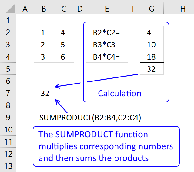
The SUMIFS function calculates a total based on multiple criteria, it has been available in Excel since version 2010. I recommend the SUMPRODUCT function if you use an earlier Excel version than 2010.
The SUMIFS function in cell D11 adds numbers from column D based on criteria applied to columns B and C.
This article explains how to use the SUMIFS function in great detail.
Table of Contents
- Syntax
- Arguments
- Example 1 - greater than
- Example 2 - not equal
- Example 3 - multiple criteria
- Example 4 - OR logic
- Example 5 - partial match
- Example 6 - how to use logical operators
- How do I sum values between n-th weekday this month and n-th weekday next month?
- Sum cells based on criteria
- Sum values between two dates and based on a condition
- Function not working
- Get Excel *.xlsx file
1. Syntax
SUMIFS(sum_range, criteria_range1, criteria1, [criteria_range2], [criteria2], ...)
2. Arguments
| sum_range | Required. A cell reference to a cell range whose numbers you want to sum. |
| criteria_range1 | Required. The cell range you want to test Criteria1 for. |
| criteria1 | Required. The condition you want to use applied to criteria_range1 to sum the corresponding cells in sum_range |
| [criteria_range2] | Optional. Up to 127 additional arguments. |
| [criteria2] | Optional. Up to 127 additional arguments. |
3. Example 1 - greater than

The image above shows the SUMIFS function cell C11, it adds numbers from C3:C8 if the corresponding number in cells B3:B8 is larger than 3. Cell B11 specifies the condition, notice the larger than character combined with number 3.
Cells B6, B7, and B8 all contain numbers higher than 3. The corresponding numbers are in cells C6, C7, and C8. These are 20 + 50 + 20 equals 90.
Formula in cell C11:
3.1 Explaining formula
Step 1 - Populate arguments
SUMIFS(sum_range, criteria_range1, criteria1, [criteria_range2], [criteria2], ...)
becomes
SUMIFS(C3:C8, B3:B8, B11)
Step 2 - Evaluate SUMIFS function
SUMIFS(C3:C8, B3:B8, B11)
becomes
SUMIFS({10; 50; 30; 20; 50; 20},{1; 2; 3; 4; 5; 6},">3")
and returns 90.
4, 5, and 6 are larger than three. The corresponding numbers on the same rows are 20, 50, and 20.
20 + 50 + 20 equals 90.
4. Example 2 - not equal

The image above demonstrates a SUMIFS function in cell C11 that adds numbers from C3:C8 if the corresponding value on the same row in cells B3:B8 are not equal to "Small".
Cell B11 specifies the condition, cells B7 and B4 meet the condition and the corresponding numbers are 50 and 50. The total is 100, 50 + 50 equals 100.
Formula in cell C11:
4.1 Explaining formula
Step 1 - Populate arguments
SUMIFS(sum_range, criteria_range1, criteria1, [criteria_range2], [criteria2], ...)
becomes
SUMIFS(C3:C8, B3:B8, B11)
Step 2 - Evaluate SUMIFS function
SUMIFS(C3:C8, B3:B8, B11)
becomes
SUMIFS({10; 50; 30; 20; 50; 20}, {"Small"; "Large"; "Small"; "Small"; "Medium"; "Small"}, "<>Small")
and returns 100. "Large" and "Medium" are not equal to Small, the corresponding values on the same rows are 50 and 50.
50 + 50 equals 100.
5. Example 3 - criteria

This section describes how to use multiple conditions in the SUMFIS function. The image above demonstrates an example with two conditions, each condition applies to a separate column.
Formula in cell D11:
5. Explaining formula
Step 1 - Populate arguments
SUMIFS(sum_range, criteria_range1, criteria1, [criteria_range2], [criteria2], ...)
becomes
SUMIFS(D3:D8, B3:B8, B11, C3:C8, C11)
Step 2 - Evaluate SUMIFS function
SUMIFS(D3:D8, B3:B8, B11, C3:C8, C11)
becomes
SUMIFS({10; 50; 30; 20; 50; 20},{101; 102; 103; 104; 105; 106},"<>104",{"Small"; "Large"; "Small"; "Small"; "Medium"; "Small"},"Small")
and returns 60. 10 + 30 + 20 equals 60.
6. Example 4 - OR logic

This example demonstrates how to sum numbers using OR logic, however, I recommend using the SUMPRODUCT function in this case. The SUMIFS function won't allow me to use functions, only cell references, in the second argument.
The formula in cell G3 uses two conditions, if any of the conditions match a value in B3:B8 the corresponding number on the same row in C3:C8 is added to a total. Cells B3, B5, B6, B7, and B8 match one of the conditions, the corresponding cells on the same rows are B3, B5, B6, B7, and B8. 10 + 30 + 20 + 50 + 20 equals 130.
Formula in cell G3:
6.1 Explaining formula
Step 1 - Identify cells equal to criteria
The COUNTIF function calculates the number of cells that is equal to a condition.
COUNTIF(range, criteria)
COUNTIF(E3:E4, B3:B8)
becomes
COUNTIF({"Small"; "Medium"}, {"Small"; "Large"; "Small"; "Small"; "Medium"; "Small"})
and returns {1; 0; 1; 1; 1; 1}.
Step 2 - Multiply array with numbers
The asterisk character lets you multiply numbers in Excel, this works fin with arrays as well.
COUNTIF(E3:E4, B3:B8)*C3:C8
becomes
{1; 0; 1; 1; 1; 1}*{10; 50; 30; 20; 50; 20}
and returns {10; 0; 30; 20; 50; 20}.
Step 2 - Add numbers and return a total
The SUMPRODUCT function calculates the product of corresponding values and then returns the sum of each multiplication.
SUMPRODUCT(array1, [array2], ...)
SUMPRODUCT(COUNTIF(E3:E4, B3:B8)*C3:C8)
becomes
SUMPRODUCT({10; 0; 30; 20; 50; 20})
and returns 130 in cell 130.
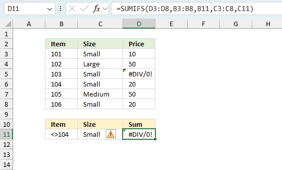
7. Example 5 - partial match
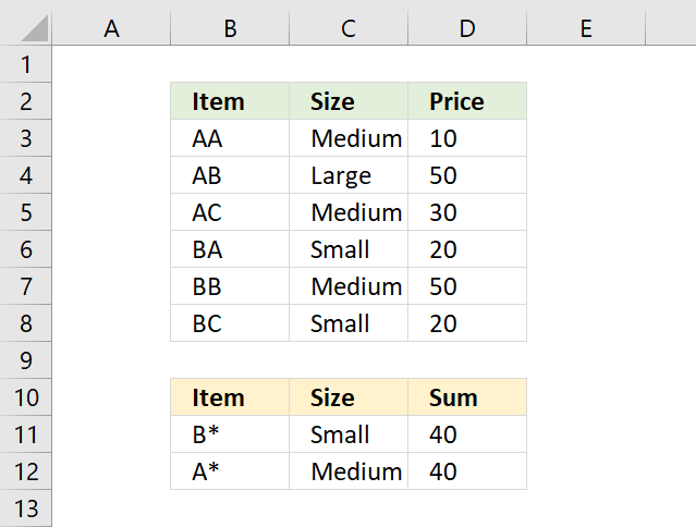
The SUMIFS function in cell D11 sums all corresponding values that begin with B in column B and is Small in column C.
You can use wildcard characters like:
- * (asterisk) - Matches any length of characters also 0 (zero)
- ? (question mark) - matches any single character
7.1 Explaining formula
Step 1 - Populate arguments
SUMIFS(sum_range, criteria_range1, criteria1, [criteria_range2], [criteria2], ...)
becomes
SUMIFS(D3:D8, B3:B8, B11, C3:C8, C11)
Step 2- Evaluate SUMIFS function
SUMIFS(D3:D8, B3:B8, B11, C3:C8, C11)
becomes
SUMIFS({10; 50; 30; 20; 50; 20},{"AA"; "AB"; "AC"; "BA"; "BB"; "BC"},"B*",{"Medium"; "Large"; "Medium"; "Small"; "Medium"; "Small"},"Small")
and returns 40 in cell D11. 20 + 20 equals 40.
8. Example 6 - How to use logical operators

The formula in cell D11 sums numbers in column D based on numbers less than 104 in column B and Small in column C.
You are also allowed to use logical operators like:
- > larger than
- < smaller than
- = equal to
- <> not equal to
- =>larger than or equal to
- =<less than or equal to
8.1 Explaining formula
Step 1 - Populate arguments
SUMIFS(sum_range, criteria_range1, criteria1, [criteria_range2], [criteria2], ...)
becomes
SUMIFS(D3:D8, B3:B8, B11, C3:C8, C11)
Step 2- Evaluate SUMIFS function
SUMIFS(D3:D8, B3:B8, B11, C3:C8, C11)
becomes
SUMIFS({10; 50; 30; 20; 50; 20},{101; 102; 103; 104; 105; 106},"<>104",{"Small"; "Large"; "Small"; "Small"; "Medium"; "Small"},"Small")
and returns 60. 10 + 30 + 20 equals 60.
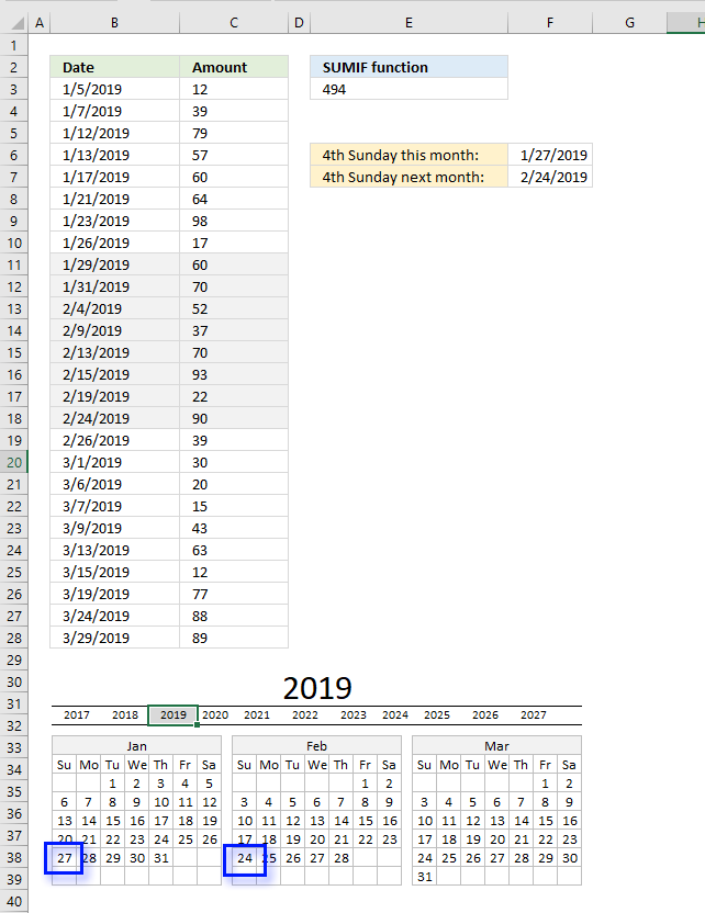
9. How do I sum values between n-th weekday this month and n-th weekday next month?
I have this formula
(=SUMIFS($C$14:$C$1000,$A$14:$A$1000,">="&DATE($A$1,8,1),$A$14:$A$1000,"<"&DATE($A$1,9,1),$F$14:$F$1000,$AA1))
which works but I want it to show from the 4th Sunday of a month to the 4th Sunday of the next month.
Formula in cell E3:
9.1 Explaining formula in cell E3
Step 1 - Calculate 4-th sunday this month
To calculate the fourth sunday we must first calculate the first Sunday in current month. Cell B3 contains this date 1/5/2019.
WEEKDAY(B3, 2) returns a number representing the weekday. 1 is Monday, 2 is Tuesday and so on.. 7 is Sunday.
WEEKDAY(B3, 2)
becomes
WEEKDAY(1/5/2019, 2)
returns 6.
7 minus 6 equals 1. We must add 1 to the date in cell B3 to get the first Sunday in that month. (This calculation works only if the date in cell B3 is less or equal to the date of the first Sunday in that month.)
B3+(7-WEEKDAY(B3, 2))+21
becomes
1/5/2019+(7-WEEKDAY(B3, 2))+21
becomes
1/5/2019+1+21
To get the fourth Sunday we add 21 to the date of the first Sunday.
1/5/2019+1+21 equals 1/27/2019.
Step 2 - Calculate 4-th sunday next month
To get the first day of the next month we need to calculate the first date of this month and then add 1 to the month.
DATE(YEAR(B3), MONTH(B3)+1, 1)
becomes
DATE(2019, 1+1, 1)
becomes
DATE(2019, 2, 1)
and returns 2/1/2019. This date is also used to calculate the fourth Sunday.
DATE(YEAR(B3), MONTH(B3)+1, 1)+(7-WEEKDAY(DATE(YEAR(B3), MONTH(B3)+1, 1), 2))+21
becomes
2/1/2019+(7-5)+21
becomes
2/1/2019+23 equals 2/24/2019.
Step 3 - Build SUMIFS function
The SUMIFS function allows you to add values based on conditions.
SUMIFS(C3:C28, B3:B28, ">="&B3+(7-WEEKDAY(B3, 2))+21, B3:B28, "<="&DATE(YEAR(B3), MONTH(B3)+1, 1)+(7-WEEKDAY(DATE(YEAR(B3), MONTH(B3)+1, 1), 2))+21)
becomes
SUMIFS(C3:C28, B3:B28, ">="&1/27/2019, B3:B28, "<="&2/24/2019)
and returns 494.
60+70+52+37+70+93+22+90 = 494
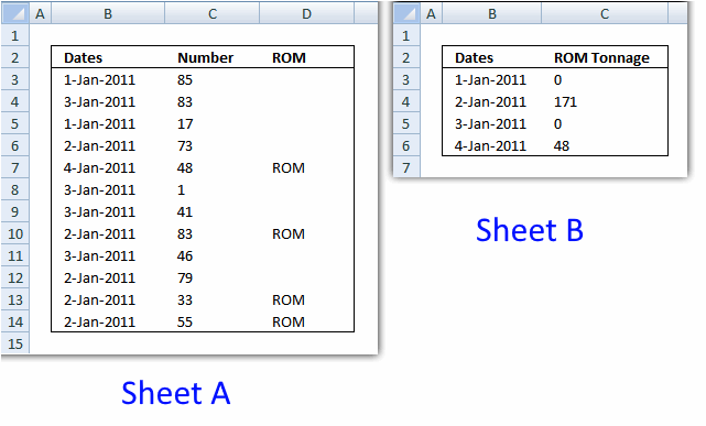
10. Sum cells based on criteria
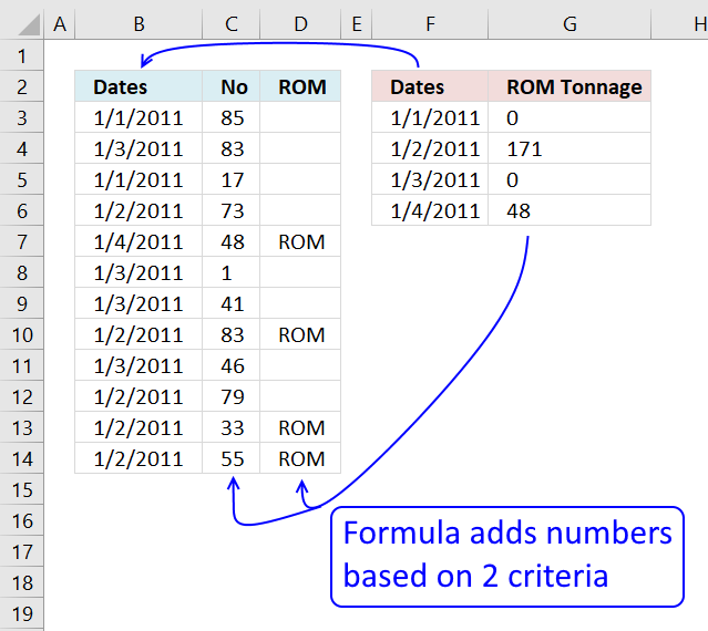
I have 57 sheets many of which are linked together by formulas, I need to get numbers from one sheet (A) into another sheet (B).
I need excel to search through the dates in sheet A to find all the data for the date that is selected on sheet B.
then I need it to search in sheet A threw the data for that specific date and select and sum all the data that is catagorised as ROM and put the total in the Cell in Sheet B called ROM Tonnage.
Answer:
I highly recommend a pivot table for this task if you have lots of data to work with. It is incredibly fast and easy to work with, however, this article demonstrates a formula.
Excel 2007 Formula in cell C3, sheet B:
The SUMIFS function lets you add numbers based on multiple conditions and returns a total, it was introduced in Excel 2007. If you own an earlier version than 2007 then see the formula below.
Excel 2003 Formula in cell C3, sheet B:
The SUMPRODUCT function is incredibly useful and easy to use, all conditions are shown in formula above.
Explaining Excel 2007 formula and later versions
SUMIFS(sum_range, criteria_range1, criteria1,..) adds the cells specified by a given set of conditions or criteria

Explaining Excel 2003 formula
Step 1 - Cells to sum

Step 2 - Find values equal to date

becomes
--({40544; 40546; 40544; 40545; 40547; 40546; 40546; 40545; 40546; 40545; 40545; 40545}=40544)
becomes
--({TRUE; FALSE; TRUE; FALSE; FALSE; FALSE; FALSE; FALSE; FALSE; FALSE; FALSE; FALSE})
and returns {1; 0; 1; 0; 0; 0; 0; 0; 0; 0; 0; 0}
Step 3 - Find values equal to criterion

becomes
--({0;0;0;0;"ROM";0;0;"ROM";0;0;"ROM";"ROM"}="ROM")
becomes
--({FALSE; FALSE; FALSE; FALSE; TRUE; FALSE; FALSE; TRUE; FALSE; FALSE; TRUE; TRUE})
and returns {0; 0; 0; 0; 1; 0; 0; 1; 0; 0; 1; 1}
Step 4 - Putting it all together
SUMPRODUCT(A!$C$3:$C$14, --(A!$B$3:$B$14=B!B3), --(A!$D$3:$D$14="ROM")))
becomes
SUMPRODUCT({85;83; 17;73; 48;1;41; 83;46;79;33;55},{1; 0; 1; 0; 0; 0; 0; 0; 0; 0; 0; 0}, {0; 0; 0; 0; 1; 0; 0; 1; 0; 0; 1; 1})
becomes
SUMPRODUCT({0; 0; 0; 0; 0; 0; 0; 0; 0; 0; 0; 0})
and returns 0 in cell C3.
Useful resources
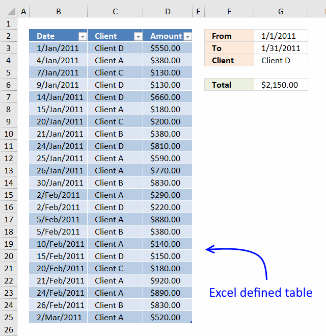
11. Sum values between two dates and based on a condition
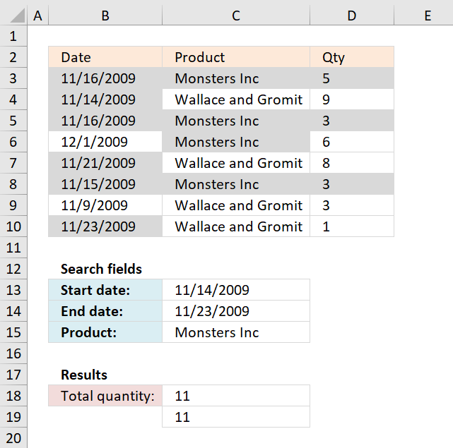
In this post, I will provide a formula to sum values in column (Qty) where a column (Date) meets two date criteria and an additional criterion in an adjacent column (Product).
I have colored the cells in column Qty that meet all criteria.
Excel formula in C18:
The SUMIFS function adds numbers based on a condition or criteria and returns a total.
SUMIFS(sum_range, criteria_range1, criteria1, [criteria_range2], [criteria2], ...)
The sum_range contains the numbers to be added: D3:D10
criteria_range1 (C3:C10) is the cell range that the criteria1 ("="&C15) will be applied to.
criteria_range2 (B3:B10) is the cell range (dates) that the criteria2 ("<="&C14) will be applied to.
criteria_range3 (B3:B10) is the cell range (dates) that the criteria3 (">="&C13) will be applied to.
SUMIFS(D3:D10, C3:C10, "="&C15, B3:B10, "<="&C14, B3:B10, ">="&C13)
Alternative formula in C19:
The SUMIFS function was introduced in Excel 2007, the SUMPRODUCT function works in all Excel versions.
Recommended post
Recommended articles
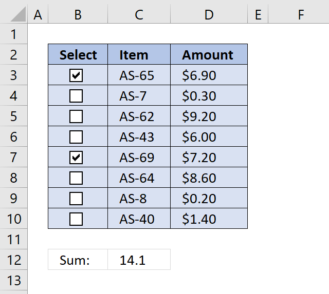
I will now demonstrate with the following table how to add check-boxes and sum enabled check-boxes using a formula. Add […]
Recommended articles
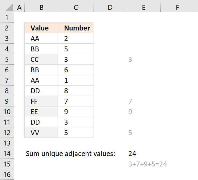
The formula in cell E14 adds a number from column C if the corresponding value in column B is unique […]
Get excel file for this tutorial
Sum values between two dates with criteria.xls
(Excel 97-2003 Workbook *.xls)
Functions in formulas above
Recommended articles
What is the SUM function? The SUM function in Excel allows you to add numerical values and returning a total, […]
Recommended articles
The SUMPRODUCT function calculates the product of corresponding values and then returns the sum of each multiplication.
Recommended articles
Farhan asks:
2254 10 20 30
2253 10 20 10
2254 10 0 51
Criteria: required 2254 sum of values b/w my specified date let say from 6-8 Nov.
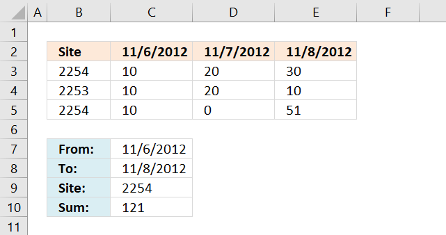
Formula in cell C10:
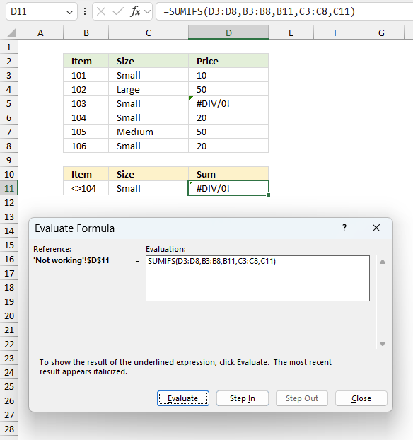
12. Function not working
The SUMIFS function
- propagates errors meaning the function returns an error if an error exists in the source data range.
- returns a #NAME! error if the function name is misspelled.
12.1 Troubleshooting the error value
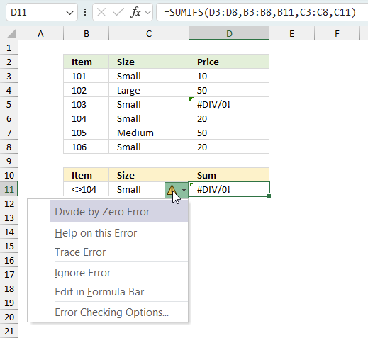
When you encounter an error value in a cell a warning symbol appears, displayed in the image above. Press with mouse on it to see a pop-up menu that lets you get more information about the error.
- The first line describes the error if you press with left mouse button on it.
- The second line opens a pane that explains the error in greater detail.
- The third line takes you to the "Evaluate Formula" tool, a dialog box appears allowing you to examine the formula in greater detail.
- This line lets you ignore the error value meaning the warning icon disappears, however, the error is still in the cell.
- The fifth line lets you edit the formula in the Formula bar.
- The sixth line opens the Excel settings so you can adjust the Error Checking Options.
Here are a few of the most common Excel errors you may encounter.
#NULL error - This error occurs most often if you by mistake use a space character in a formula where it shouldn't be. Excel interprets a space character as an intersection operator. If the ranges don't intersect an #NULL error is returned. The #NULL! error occurs when a formula attempts to calculate the intersection of two ranges that do not actually intersect. This can happen when the wrong range operator is used in the formula, or when the intersection operator (represented by a space character) is used between two ranges that do not overlap. To fix this error double check that the ranges referenced in the formula that use the intersection operator actually have cells in common.
#SPILL error - The #SPILL! error occurs only in version Excel 365 and is caused by a dynamic array being to large, meaning there are cells below and/or to the right that are not empty. This prevents the dynamic array formula expanding into new empty cells.
#DIV/0 error - This error happens if you try to divide a number by 0 (zero) or a value that equates to zero which is not possible mathematically.
#VALUE error - The #VALUE error occurs when a formula has a value that is of the wrong data type. Such as text where a number is expected or when dates are evaluated as text.
#REF error - The #REF error happens when a cell reference is invalid. This can happen if a cell is deleted that is referenced by a formula.
#NAME error - The #NAME error happens if you misspelled a function or a named range.
#NUM error - The #NUM error shows up when you try to use invalid numeric values in formulas, like square root of a negative number.
#N/A error - The #N/A error happens when a value is not available for a formula or found in a given cell range, for example in the VLOOKUP or MATCH functions.
#GETTING_DATA error - The #GETTING_DATA error shows while external sources are loading, this can indicate a delay in fetching the data or that the external source is unavailable right now.
12.2 The formula returns an unexpected value
To understand why a formula returns an unexpected value we need to examine the calculations steps in detail. Luckily, Excel has a tool that is really handy in these situations. Here is how to troubleshoot a formula:
- Select the cell containing the formula you want to examine in detail.
- Go to tab “Formulas” on the ribbon.
- Press with left mouse button on "Evaluate Formula" button. A dialog box appears.
The formula appears in a white field inside the dialog box. Underlined expressions are calculations being processed in the next step. The italicized expression is the most recent result. The buttons at the bottom of the dialog box allows you to evaluate the formula in smaller calculations which you control. - Press with left mouse button on the "Evaluate" button located at the bottom of the dialog box to process the underlined expression.
- Repeat pressing the "Evaluate" button until you have seen all calculations step by step. This allows you to examine the formula in greater detail and hopefully find the culprit.
- Press "Close" button to dismiss the dialog box.
There is also another way to debug formulas using the function key F9. F9 is especially useful if you have a feeling that a specific part of the formula is the issue, this makes it faster than the "Evaluate Formula" tool since you don't need to go through all calculations to find the issue..
- Enter Edit mode: Double-press with left mouse button on the cell or press F2 to enter Edit mode for the formula.
- Select part of the formula: Highlight the specific part of the formula you want to evaluate. You can select and evaluate any part of the formula that could work as a standalone formula.
- Press F9: This will calculate and display the result of just that selected portion.
- Evaluate step-by-step: You can select and evaluate different parts of the formula to see intermediate results.
- Check for errors: This allows you to pinpoint which part of a complex formula may be causing an error.
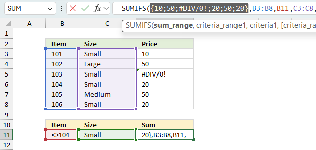
The image above shows cell reference D3:D8 converted to hard-coded value using the F9 key. The SUMIFS function requires non-error values which is not the case in this example. We have found what is wrong with the formula.
Tips!
- View actual values: Selecting a cell reference and pressing F9 will show the actual values in those cells.
- Exit safely: Press Esc to exit Edit mode without changing the formula. Don't press Enter, as that would replace the formula part with the calculated value.
- Full recalculation: Pressing F9 outside of Edit mode will recalculate all formulas in the workbook.
Remember to be careful not to accidentally overwrite parts of your formula when using F9. Always exit with Esc rather than Enter to preserve the original formula. However, if you make a mistake overwriting the formula it is not the end of the world. You can “undo” the action by pressing keyboard shortcut keys CTRL + z or pressing the “Undo” button
12.3 Other errors
Floating-point arithmetic may give inaccurate results in Excel - Article
Floating-point errors are usually very small, often beyond the 15th decimal place, and in most cases don't affect calculations significantly.
Get excel *.xlsx file
'SUMIFS' function examples
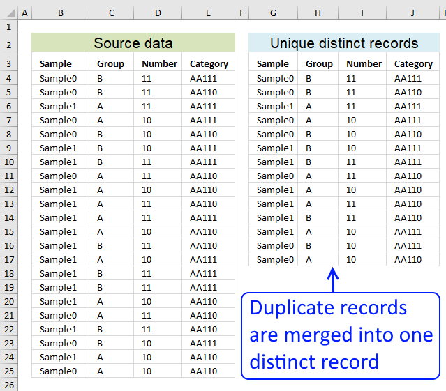
Table of contents Filter unique distinct row records Filter unique distinct row records but not blanks Filter unique distinct row […]
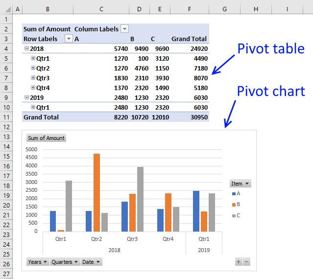
A pivot table allows you to examine data more efficiently, it can summarize large amounts of data very quickly and is very easy to use.
Andrew asks: LOVE this example, my issue/need is, I need to add the results. So instead of States and Names, […]
Functions in 'Math and trigonometry' category
The SUMIFS function function is one of 62 functions in the 'Math and trigonometry' category.
Excel function categories
Excel categories
38 Responses to “How to use the SUMIFS function”
Leave a Reply
How to comment
How to add a formula to your comment
<code>Insert your formula here.</code>
Convert less than and larger than signs
Use html character entities instead of less than and larger than signs.
< becomes < and > becomes >
How to add VBA code to your comment
[vb 1="vbnet" language=","]
Put your VBA code here.
[/vb]
How to add a picture to your comment:
Upload picture to postimage.org or imgur
Paste image link to your comment.
Thanks!
I'm in a similar situation as the example above, but I have three sheets and three conditions. Sheet1 has three columns: Site, Quarter, Boxes; Sheet2 has two columns: Site, Designation; and Sheet 3 has three columns: Designation, Quarter, Boxes. I want to sum the last column (boxes) in Sheet1 to the last column(boxes) in Sheet3 based on criteria in all three sheets.
The common links between the sheets are Sheet1-Sheet2: Site, Sheet2-Sheet3: Designation, Sheet1-Sheet3: Quarter. I having difficulty getting it to sum only facilities with a certain Designation for a given Quarter. I am trying to use SUMIFS but am not sure if this is the appropriate formula. Any thoughts on how I can make this work?
klm,
I am not sure I understand. Check out the file I created:
klm.xlsx
Thanks you saved alot of time for me
THanks buddy.... grt work.....
am i right in thinking that there shouldn't be a semi-colon after C3:C10. I removed it and put a comma instead and it worked
=SUMIFS(D3:D10, C3:C10;"="&C15, B3:B10, "="&C13) + ENTER
huw bevan,
Thanks for letting me know!
Site 6-Nov-12 7-Nov-12 8-Nov-12
2254 10 20 30
2253 10 20 10
2254 10 0 51
Criteria: required 2254 sum of values b/w my specified date let say from 6-8 Nov.
Farhan,
I added your question and the answer to this post.
Thanks for commenting!
Thank you so much for posting this. I had been wrestling with this issue for many, many hours, and your solution and explanation were by far the clearest and best I've seen. Thanks for sharing the knowledge!
Thank ..... It was really useful
Can you post an excel sheet containing top 50 of your solution??
Thank's
How to use it with filter date?
Good Day
Thanks so much for this information. I was working on this problem for about 4 hours before doing a search and finding this. It solved my problem immediately and perfectly !!!
JDC,
Thank you!
thanks you so much n thanks for your sharing
Thanks. You are the only one I have found that puts the cell-headers on their photos and even provides the example file! This fixed my headaches in less than 10 minutes for 3 of these calculations! Thanks again!
how can sum value with date criteria on another worksheet?
kisembo,
Original formula:
Change cell references!
Hi;
I google a lot, I found your website here. finally I got solution with simple explanation from you for my problem sum-total between two dates with category.
and much more to be explore from your site about excel it very helpful. thanks.
Yudi,
thank you!
The formula works for one range, but when applying to another date range, nothing is returned.
I have created new cells for other ranges and inserted them into the formula, but nothing is returned.
What do you suggest?
Ryan Chatt
What happens when you evaluate the formula?
1. Go to tab "Formulas"
2. Press with left mouse button on "Evaluate Formula" button
3. Press with left mouse button on Evaluate button repeatedly to see where the error is.
what if I need to reference another sheet (for the transaction value) AND use the SUMPRODUCT formula ?
How would I do that ??
Thanks!
Many thanks just what I have been searching for :-)
I get a #VALUE! error when applying the formula...evaluating the error shows that the dates are not recognized, coming up with #NAME? related to values in H22 and I22.
=SUMIFS('INVENTORY RECEIVED'!$P$8:$NP$228,'INVENTORY RECEIVED'!$D$8:$D$228,"="&C25,'INVENTORY RECEIVED'!$P$7:$NP$7,”=”&$H$22)
C25 (Sheet 1) = cell with product name trying to get the sum for between date range listed
I22 (Sheet 1) = Date Range End (31-Mar-2017)
H22 (Sheet 1) = Date Range Begin (01-Jan-2017)
P7:NP7 (Inventory Received) = row & columns with daily dates (Jan 1 - Dec 31)
P8:NP228 (Inventory Received) = cell range with values to sum
D8:D228 (Inventory Received) = column with product names to lookup
So, in the 'Master File' (Sheet 1), I want to find out how many items were purchased for product named in cell C25 between dates I22 and H22, listed in the table on sheet 'Inventory Received' within the data range P8:NP228...
Thanks!
Sorry, this is the formula:
=SUMIFS('INVENTORY RECEIVED'!$P$8:$NP$228,'INVENTORY RECEIVED'!$D$8:$D$228,"="&C25,'INVENTORY RECEIVED'!$P$7:$NP$7,”=”&$H$22)
Hi Oscar,
Not sure what is happening and why the formula keeps getting truncated when pasting...Writing the formula in its individual parts, hopefully this works...
=SUMIFS('INVENTORY RECEIVED'$P$8:$NP$228,
'INVENTORY RECEIVED'!$D$8:$D$228,
"="&C25,
'INVENTORY RECEIVED'!$P$7:$NP$7,
"="&$H$22)
In the Excel formula evaluator, the $I$22 and $H$22 return #NAME? errors, though the $P$7:$NP$7 range returns the dates listed (in 42736 format)...Thanks again.
That didn't work either...never mind.
Amazing Farhan thank you. your formula support for my excel file workings
Thank you so much for this!! I could not find this anywhere online. We use a Google Doc Form where employees submit their PTO requests using the values:
- Name/Email
- PTO Start Date (all years)
- Number of weekdays they will be off
I used your formula to total the number of days taken per year per employee and worked perfectly!
Screenshot: https://postimg.cc/LY5dt85j
So awesome! Thank you!
Hello excel gurus,
Based on table 1, is there a way to calculate the number of tasks a given resource (who) is assigned and working for each calendar day (table 2). I've given a tried using sumproduct or countifs but I haven't found the way to get the desirable results.
I will appreciate any insight about it.
Thanks!
table 1:
task_name who start_dt end_dt
task1 CR 1/8/2021 1/8/2021
task2 MS 1/8/2021 1/9/2021
task3 CR 1/8/2021 1/11/2021
task4 CR 1/13/2021 1/15/2021
table 2:
1/7/2021 1/8/2021 1/9/2021 1/10/2021 1/11/2021 1/12/2021 1/13/2021 1/14/2021 1/15/2021
CR 0 2 1 1 1 0 1 1 1
MS 0 1 1 0 0 0 0 0 0
I just figured out what was the issue. Using sumproduct formula, I had forgotten to include ctrl +shift + enter at the end.
e.g.
=SUMPRODUCT(($K$2:$K$5=O$1)*($J$2:$J$5=$N2)) then CTRL+SHIFT+ENTER
Thanks anyway!
I want to thank you SO MUCH for this! You have no idea how much you helped me!
ANA MARIA
You are welcome!
Oscar, you have no idea how much I have been searching for a way to do what your example of SUMPRODUCT did. I was always looking for SUMIF, SUMIFS, INDEX/MATCH, XLOOKUP hoping to get the right result but no luck until now. Thank you so much for this tutorial. You have helped me out tremendously.
Thank you Sam!