Create dependent drop down lists containing unique distinct values

Table of Contents
- Create dependent drop down lists containing unique distinct values - Excel 365
- Create dependent drop down lists containing unique distinct values
- Create dependent drop down lists containing unique distinct values in multiple rows
- Create a drop down list containing alphabetically sorted values
- Dependent drop down lists - Enable/Disable selection filter
- Dependent drop-down lists in multiple rows
- Use a drop down list to filter and concatenate unique distinct values
1. Create dependent drop down lists containing unique distinct values - Excel 365
Creating dependent drop down lists in Excel 365 is much easier than older Excel versions. No need for "named ranges" or the OFFSET function. In fact, the formulas needed to build this are also much smaller and easier to work with.
What is a drop down list?
Drop down list is one of the features in the Excel's "Data Validation" toolbox, it allows you to select a value from a given list of values. It works like this, you select the cell containing the drop down list. A grey box containing a arrow pointing down appears, press the grey box with the left mouse button and the list shows up. Press with left mouse button an any of the values in the list to select it.
What is a dependent drop down list?
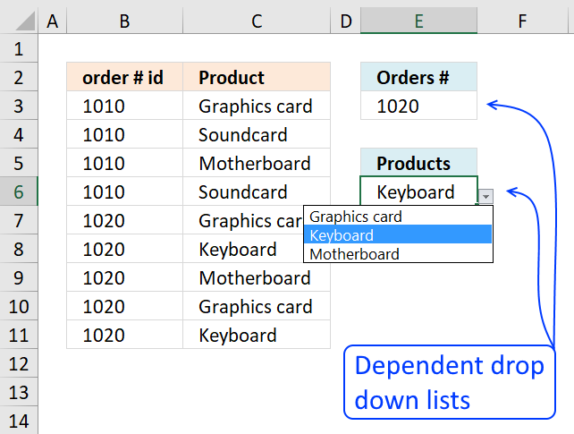
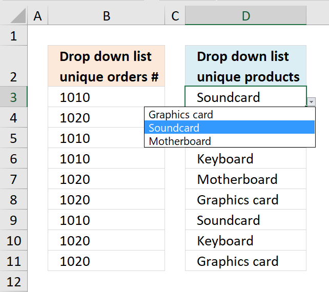
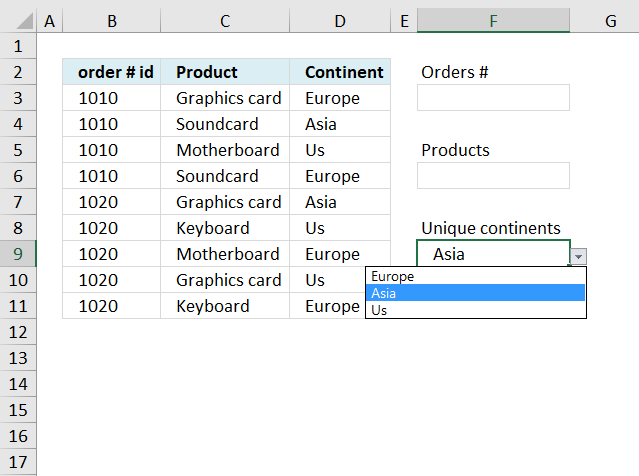
Dependent drop down lists changes based on the selected values, this tutorial uses only two drop down lists. The second drop down list shows values based on what the selected value is in the first drop down list. The data table contains the "rules" for which values to display. For example, order 1030, in the image above has only one product which is "keyboard", see row 10. This means that only one value is shown in the second drop down list if 1030 is selected in the first drop down list. However, if order "1020" is selected in the first drop down then the second drop down lists three products "Graphics card", "Keyboard" , and "Motherboard", see the image above.
I have located the calculations (E4:F4) on the same worksheet as the data table (B3:C11) and drop down lists (B14 and C14) to simplify the demonstration. I recommend you put the calculations on a separate worksheet.
Excel 365 dynamic array formula in cell E4:
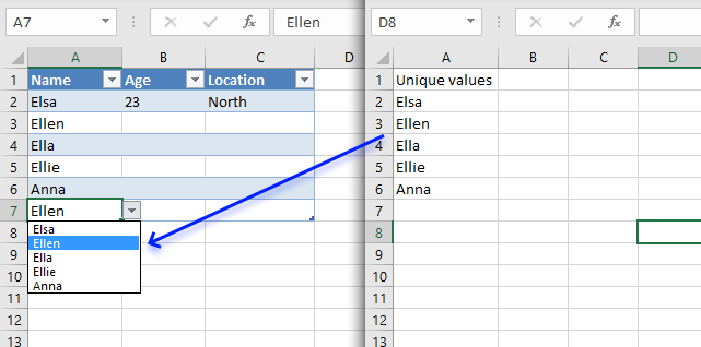
The formula above lists unique distinct values using B3:B11 as the data source. The formula spills the values to cell E4 and cells below automatically.
These values will populate the first drop down list in cell B14, it it now time to build the first drop down list.
What are unique distinct values?
Unique distinct values are all values, however, duplicates are merged in to one distinct value. This means that the list contains only one instance of each value, all duplicates are gone.
Drop down list in cell B14:
- Select cell B14
- Go to tab "Data" on the ribbon.
- Press with left mouse button on the "Data Validation" button on the ribbon.
A dialog box appears. - Press with left mouse button on the "Allow:" field.
A drop down list expands, select "List". - Press with left mouse button on the "Source:" field.
Type =E4#
E4# is a cell reference to an Excel 365 dynamic array formula.

- Press the "OK" button to dismiss the dialog box and apply changes.
Excel 365 dynamic array formula in cell F4:
The formula in cell F4 uses the selected value in B14 to filter the corresponding values from column "Products" in the data table C3:C11.
Explaining the formula in cell F4
Step 1 - Create logical expression
The equal sign lets you compare value to values, the result is a boolean value TRUE or FALSE.
B14=B3:B11
returns {FALSE; FALSE; FALSE; ... ; TRUE}
Step 2 - Filter values
The FILTER function extracts values/rows based on a condition or criteria.
Function syntax: FILTER(array, include, [if_empty])
FILTER(C3:C11,B14=B3:B11)
returns {"Graphics card"; "Keyboard"; "Motherboard"; "Keyboard"}
Step 3 - List unique distinct values based on filtered list
The UNIQUE function returns a unique or unique distinct list.
Function syntax: UNIQUE(array,[by_col],[exactly_once])
UNIQUE(FILTER(C3:C11,B14=B3:B11))
becomes
UNIQUE({"Graphics card";"Keyboard";"Motherboard";"Keyboard"})
and returns
{"Graphics card";"Keyboard";"Motherboard"}
Drop down list in cell C14:
- Select cell C14
- Go to tab "Data" on the ribbon.
- Press with left mouse button on the "Data Validation" button on the ribbon.
A dialog box appears. - Press with left mouse button on the "Allow:" field.
A drop down list expands, select "List". - Press with left mouse button on the "Source:" field.
Type =F4#
F4# is a cell reference to an Excel 365 dynamic array formula.

- Press the "OK" button to dismiss the dialog box and apply changes.
You can easily expand the number of drop down lists, you need the same number of calculations as drop down lists.
Limitations
- The major limitation is that it is not possible to use dependent drop down lists in multiple rows, each row contains a group of dependent drop down lists.
What to do: A VBA macro explained in section 3 below. - Another disadvantage is that the drop down lists doesn't clear their values when new values are selected. For example, lets say the first drop down contains value "1020" and the second drop down contains "Keyboard" if you now change the value in the first drop down to "1030" the second drop down doesn't change or clear automatically. In fact, the second value "Keyboard" is not a valid value based on the selected value in the first drop down list.
Solution: Use conditional formatting to highlight cells perhaps red to inform users that a value is invalid. - The drop down lists are easy to delete, perhaps too easy. For example, if you copy cell B15 and paste it to B14 the drop down list in B14 is now gone without any warning. A quick fix is to "Undo" the action however most users may not even notice what they have done since no warning was issued.
Solution: Use borders around cells to indicate they are special and contain drop down lists. Another solution is to use a vba macro that restricts user from deleting the drop down list.
Get Excel 365 *.xlsx file
unique distinct dependent listsv2.xlsx
2. Create dependent drop down lists containing unique distinct values
This article explains how to build dependent drop down lists.
Here is a list of order numbers and products.

We are going to create two drop-down lists.
The first drop down list contains unique distinct values from column A.
The second drop-down list contains unique distinct values from column B, based on the chosen value in the first drop-down list.
Watch a video on how to set up dependent drop-down lists
Create a dynamic named range
A named range is great for lists that expand, however I recommend an Excel defined table if you have Excel 2007 or a later version.
- Press with left mouse button on "Formulas" tab
- Press with left mouse button on "Name Manager"
- Press with left mouse button on "New..."
- Type a name. I named it "order". (See attached file at the end of this post)
- Type =OFFSET(Sheet1!$A$2,0,0,COUNTA(Sheet1!$A$2:$A$1000)) in "Refers to:" field.
- Press with left mouse button on "Close" button
Recommended article
Recommended articles
What is a named range? A named range is a feature in Excel that allows you to assign a specific […]
Create a unique distinct list from column A
- Select Sheet2
- Select cell A2
- Type "=INDEX(order,MATCH(0,COUNTIF($A$1:A1,order),0))" + CTRL + SHIFT + ENTER
- Copy cell A2 and paste it down as far as needed.
Recommended article:
Recommended articles

First, let me explain the difference between unique values and unique distinct values, it is important you know the difference […]
Create a dynamic named range to get unique distinct list
- Select Sheet2
- Press with left mouse button on "Formulas" tab
- Press with left mouse button on "Name Manager"
- Press with left mouse button on "New..."
- Type a name. I named it "uniqueorder". (See attached file at the end of this post)
- Type =OFFSET(Sheet2!$A$2, 0, 0, COUNT(IF(Sheet2!$A$2:$A$1000="", "", 1)), 1) in "Refers to:" field.
- Press with left mouse button on "Close" button
Recommended article:
Recommended articles
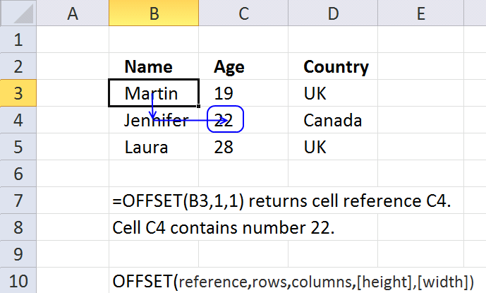
What is the OFFSET function? The OFFSET function returns a reference to a range that is a given number of […]
Recommended articles
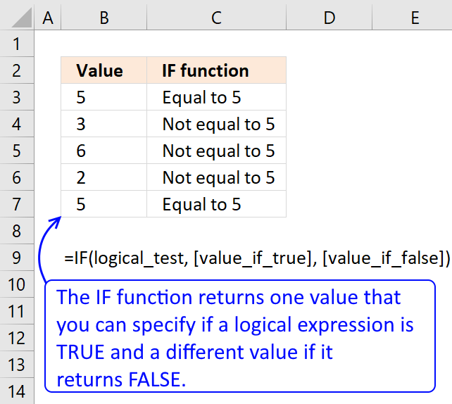
Checks if a logical expression is met. Returns a specific value if TRUE and another specific value if FALSE.
Create drop down list
- Select Sheet1
- Select cell D2
- Press with left mouse button on Data tab
- Press with left mouse button on Data validation button
- Press with left mouse button on "Data validation..."
- Select List in the "Allow:" window.
- Type =uniqueorder in the "Source:" window
- Press with left mouse button on OK!
Here is a picture of what we have accomplished so far.

Recommended article
Recommended articles
A drop-down list in Excel prevents a user from entering an invalid value in a cell. Entering a value that […]
How to create a secondary unique list based on only one chosen cell value in first drop down list
Create a dynamic named range
- Press with left mouse button on "Formulas" tab
- Press with left mouse button on "Name Manager"
- Press with left mouse button on "New..."
- Type a name. I named it "product". (See attached file at the end of this post)
- Type =OFFSET(Sheet1!$B$2,0,0,COUNTA(Sheet1!$B$2:$B$1000)) in "Refers to:" field.
- Press with left mouse button on "Close" button
Create a unique distinct list from column B
- Select Sheet2
- Select cell B2
- Type "=INDEX(product, MATCH(0, COUNTIF($B$1:B1, product)+(order<>Sheet1!$D$2), 0))" + CTRL + SHIFT + ENTER
- Copy cell B2 and paste it down as far as needed.
Create a dynamic named range to get unique distinct list
- Select Sheet2
- Press with left mouse button on "Formulas" tab
- Press with left mouse button on "Name Manager"
- Press with left mouse button on "New..."
- Type a name. I named it "uniqueproduct". (See attached file at the end of this post)
- Type =OFFSET(Sheet2!$B$2, 0, 0, COUNT(IF(Sheet2!$B$2:$B$1000="", "", 1)), 1) in "Refers to:" field.
- Press with left mouse button on "Close" button
Create drop down list
- Select Sheet1
- Select cell D5
- Press with left mouse button on Data tab
- Press with left mouse button on Data validation button
- Press with left mouse button on "Data validation..."
- Select List in the "Allow:" window.
- Type =uniqueproduct in the "Source:" window
- Press with left mouse button on OK!

Get example workbook
unique distinct dependent lists.xls
(Excel 97-2003 Workbook *.xls)
Get example workbook with a third column of data
unique-distinct-dependent-lists1 three columns.xls
(Excel 97-2003 Workbook *.xls)
3. Create dependent drop down lists containing unique distinct values in multiple rows
How can i use these list for multiple rows?
I would like to use these lists for multiple rows and let people enter detailed records.
Answer:
In my example workbook, I have created three sheets:
- Multiple rows
- Data
- Calculation
The selected drop-down list gets all values from a single column on sheet "Calculation".
The array formula on sheet "Calculation" has to "know" which cell you have selected and the adjacent cell value on sheet "Multiple rows".

Setup an automatic event on sheet "Multiple rows" (VBA)
- Press Alt-F11 to open VB editor
- Double press with left mouse button on Sheet1 "Multiple rows" in project window.
- Copy and paste vba code below into code window.
Private Sub Worksheet_SelectionChange(ByVal Target As Range)
Sheets("Calculation").Range("D1") = Sheets("Multiple rows").Range("A" & ActiveCell.Row)
End Sub
Cell D1 on sheet "Calculation" is updated instantly whenever you select a cell on sheet "Multiple rows"
Setting up the "Calculation" sheet
Array formula in cell B2:
To enter an array formula, type the formula in a cell then press and hold CTRL + SHIFT simultaneously, now press Enter once. Release all keys.
The formula bar now shows the formula with a beginning and ending curly bracket telling you that you entered the formula successfully. Don't enter the curly brackets yourself.
Copy cell B2 and paste it down as far as needed. You can read how this formula works here: 5 easy ways to extract unique distinct values

4. Create a drop down list containing alphabetically sorted values
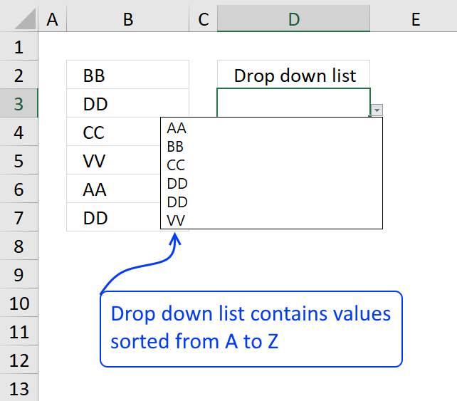
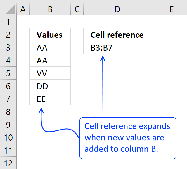
This section describes how to create a drop-down list populated with sorted values from A to Z. The sorted list is dynamic and it adds new values as you type them. The picture below shows a list containing some random values.

First we need to build a cell reference that expands when we add values to the list, named ranges allow us to do that.
However, if you own Excel 2007 or a later version I highly recommend using an Excel defined table instead.
It has a built-in dynamic cell reference system, named structured referencing.
4.1 Create a dynamic named range "List"
The following instructions tells you how to build an automatically expanding cell range.
- Press with left mouse button on "Formulas" tab
- Press with left mouse button on "Name Manager"
- Press with left mouse button on "New..."
- Type a name. I named it "List". (See attached file at the end of this post)
- Type
=OFFSET(Sheet1!$A$1, 0, 0, COUNTA(Sheet1!$A$1:$A$1001))
in "Refers to:" field.
- Press with left mouse button on "Close" button

Want to learn more about named ranges? Read this:
Recommended articles
What is a named range? A named range is a feature in Excel that allows you to assign a specific […]
4.2 Create a dynamic list sorted from A to Z
- Select Sheet2
- Select cell A1
- Type
=IF(COUNTA(List)>=ROWS($A$2:A2), INDEX(List, MATCH(SMALL(COUNTIF(List, "<"&List), ROW(A1)), COUNTIF(List, "<"&List), 0)), "") + CTRL + SHIFT + ENTER
- Copy cell A2 and paste it down as far as needed.

This article explains how to extract a unique distinct list sorted alphabetically:
Recommended articles
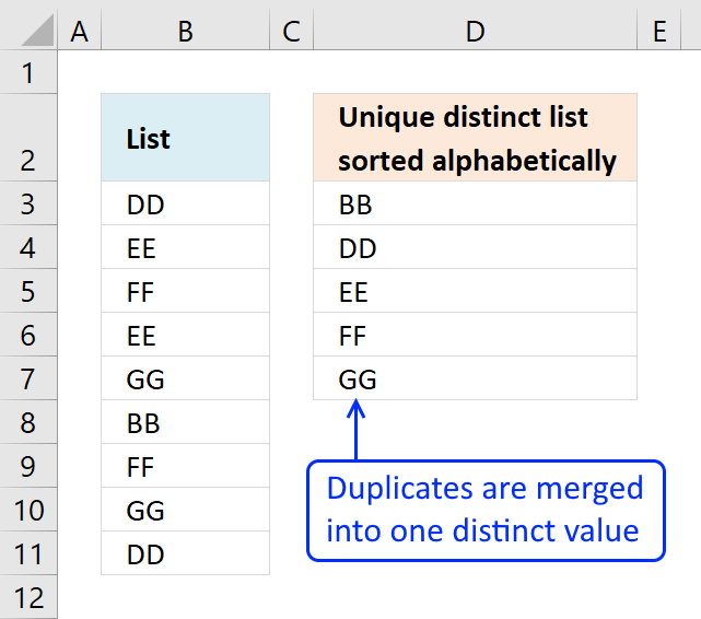
This article demonstrates Excel formulas that allows you to list unique distinct values from a single column and sort them […]
You can even use a condition if you prefer, read more here:
Recommended articles
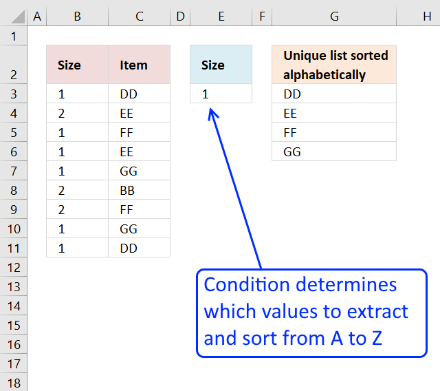
This article demonstrates how to extract unique distinct values based on a condition and also sorted from A to z. […]
4.3 Create a dynamic named range "SortedValues"
- Press with left mouse button on "Formulas" tab
- Press with left mouse button on "Name Manager"
- Press with left mouse button on "New..."
- Type a name. I named it "SortedValues". (See attached file at the end of this post)
- Type
=OFFSET(Sheet2!$A$1, 0, 0, COUNTA(Sheet2!$A$1:$A$1001))
in "Refers to:" field.
- Press with left mouse button on "Close" button

Learn more about the function OFFSET function:
Recommended articles
What is the OFFSET function? The OFFSET function returns a reference to a range that is a given number of […]
4.4 How to create a drop down list containing dynamic values
- Press with left mouse button on Data tab
- Press with left mouse button on Data validation button
- Press with left mouse button on "Data validation..."
- Select List in the "Allow:" window. See picture below.
- Type
=SortedValues
in the "Source:" window
- Press with left mouse button on OK!

If you are using an excel defined table, read this:
Recommended articles
This article demonstrates different ways to reference an Excel defined Table in a drop-down list and Conditional Formatting formulas. The […]
5. Dependent drop down lists - Enable/Disable selection filter
I have this working right now with 6 drop downs/lists. I wanted to see if you possibly know of a way to see additional information in drop down #4 if there are no selections in drop down #2 and #3.
Currently, I have hemisphere in drop down 1, Sector in drop down 2, Region in drop down 3, and Area is drop down 4.
If I select a value in drop down #1 (Hemisphere), I would like to see what areas I can filter on in drop down #4 without having to select values in drop down 2 and 3.
Is there a way to make that work?
Answer:
Yes, I have simplified my answer to three drop down lists. I recommend geting the attached excel file before reading this post.

5.1 Setup and create first drop down list
5.1.1 Create a dynamic named range
- Press with left mouse button on "Formulas" tab
- Press with left mouse button on "Name Manager"
- Press with left mouse button on "New..."
- Type a name. I named it "order". (See attached file at the end of this post)
- Type =OFFSET(Sheet1!$A$2,0,0,COUNTA(Sheet1!$A$2:$A$1000)) in "Refers to:" field.
- Press with left mouse button on "Close" button
5.1.2 Create a unique distinct list from column A, Sheet1
- Select Sheet2
- Select cell A3. (Cell A2 is empty)
- Type =INDEX(order,MATCH(0,COUNTIF($A$1:B2,order),0)) + CTRL + SHIFT + ENTER. This is an array formula!!
- Copy cell A3 and paste it down as far as needed.
Sheet 2

5.1.3 Create a dynamic named range to get unique distinct list
- Select Sheet2
- Press with left mouse button on "Formulas" tab
- Press with left mouse button on "Name Manager"
- Press with left mouse button on "New..."
- Type a name. I named it "uniqueorder".
- Type =OFFSET(Sheet2!$A$2, 0, 0, COUNT(IF(Sheet2!$A$3:$A$1000="", "", 1))+1, 1) in "Refers to:" field.
- Press with left mouse button on "Close" button
5.1.4 Create drop down list
- Select Sheet1
- Select cell E2
- Press with left mouse button on Data tab
- Press with left mouse button on Data validation button
- Press with left mouse button on "Data validation..."
- Select List in the "Allow:" window.
- Type =uniqueorder in the "Source:" window
- Press with left mouse button on OK!
5.2 Setup and create second dependent drop down list
5.2.1 Create a dynamic named range
- Select sheet1
- Press with left mouse button on "Formulas" tab
- Press with left mouse button on "Name Manager"
- Press with left mouse button on "New..."
- Type a name. I named it "product". (See attached file at the end of this post)
- Type =OFFSET(Sheet1!$B$2,0,0,COUNTA(Sheet1!$B$2:$B$1000)) in "Refers to:" field.
- Press with left mouse button on "Close" button
5.2.2 Create a unique distinct list from column B, sheet1.
- Select Sheet2
- Select cell B3. (Cell B2 is empty.)
- Type =INDEX(product, MATCH(0, COUNTIF($B$1:B2, product)+IF(Sheet1!$E$2<>0, order<>Sheet1!$E$2, order=""), 0)) + CTRL + SHIFT + ENTER. This is an array formula!!
- Copy cell B3 and paste it down as far as needed.
Sheet2

5.2.3 Create a dynamic named range to get unique distinct list
- Select Sheet2
- Press with left mouse button on "Formulas" tab
- Press with left mouse button on "Name Manager"
- Press with left mouse button on "New..."
- Type a name. I named it "uniqueproduct".
- Type =OFFSET(Sheet2!$B$2, 0, 0, COUNT(IF(Sheet2!$B$3:$B$1000="", "", 1))+1, 1) in "Refers to:" field.
- Press with left mouse button on "Close" button
5.2.4 Create drop down list
- Select Sheet1
- Select cell E5
- Press with left mouse button on Data tab
- Press with left mouse button on Data validation button
- Press with left mouse button on "Data validation..."
- Select List in the "Allow:" window.
- Type =uniqueproduct in the "Source:" window
- Press with left mouse button on OK!
5.3 Setup and create third dependent drop down list
5.3.1 Create a dynamic named range
- Select sheet1
- Press with left mouse button on "Formulas" tab
- Press with left mouse button on "Name Manager"
- Press with left mouse button on "New..."
- Type a name. I named it "continent".
- Type =OFFSET(Sheet1!$C$2, 0, 0, COUNTA(Sheet1!$C$2:$C$1000))in "Refers to:" field.
- Press with left mouse button on "Close" button
5.3.2 Create a unique distinct list from column C, Sheet1
- Select Sheet2
- Select cell C3. (Cell C2 is empty)
- Type =INDEX(continent, MATCH(0, COUNTIF($C$1:C1, continent)+(Sheet1!$E$2<>0)*(order<>Sheet1!$E$2)+(Sheet1!$E$5<>0)*(product<>Sheet1!$E$5), 0)) + CTRL + SHIFT + ENTER. This is an array formula!!
- Copy cell C3 and paste it down as far as needed.
Sheet 2

5.3.3 Create a dynamic named range to get unique distinct list
- Select Sheet2
- Press with left mouse button on "Formulas" tab
- Press with left mouse button on "Name Manager"
- Press with left mouse button on "New..."
- Type a name. I named it "uniquecontinent".
- Type =OFFSET(Sheet2!$C$2, 0, 0, COUNT(IF(Sheet2!$C$2:$C$1000="", "", 1)), 1) in "Refers to:" field.
- Press with left mouse button on "Close" button
5.3.4 Create drop down list
- Select Sheet1
- Select cell E8
- Press with left mouse button on Data tab
- Press with left mouse button on Data validation button
- Press with left mouse button on "Data validation..."
- Select List in the "Allow:" window.
- Type =uniquecontinent in the "Source:" window
- Press with left mouse button on OK!
Example picture sheet1, first drop down list is blank and second drop down list contains all unique values.

6. Dependent drop-down lists in multiple rows
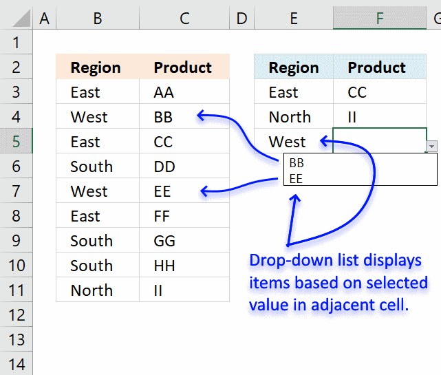
This article demonstrates how to set up dependent drop-down lists in multiple cells. The drop-down lists are populated based on the adjacent value on the same row, in other words, they are dependent on each other. Select Region "East" demonstrated above and you can only select Products "BB" and "EE", the table in cell range B2:C11 determines how they are related.
Regular drop-down lists used here are easy to insert and customize, the formulas in this workbook are easy to create and so are the named ranges as well. I will in detail explain how they work.
The downside with this approach is that you can only use two connected drop-down lists. For example, three dependent drop-down lists actually require a three-dimensional table which is possible using VBA, however, outside the scope of this article. Note, to be clear, there is no VBA code in the example demonstrated here.
Another downside with regular drop-down lists is that if you select a Region value and then a Product value and then go back and change the Region value to another value the Product value stays the same. It would have been better if that value became blank in those occasions.
It is also possible to paste a value and overwrite the drop-down list, this is how they are designed and nothing I can do about more than using perhaps VBA code or Event code to prevent such scenarios.
Check out the Dependent Drop Down lists Add-In if you need more than two dependent drop-down lists.
How I built this workbook
Cell range B2:C11 contains an Excel defined Table that automatically expands or shrinks when values are added or deleted respectively, you don't need to adjust cell references each time you edit the Excel defined Table which is a huge time saver.
There is also another data set, shown below, that is built using two array formulas. The data set extracts items (Products) for each possible value (Region) which makes it easier to populate the drop-down lists using only formulas and named ranges.
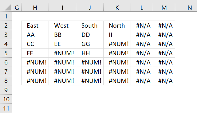
This table is dynamic and changes instantly whenever the source table is edited. Don't worry, I will explain the table above and the formulas used later in this article.
Excel defined Table
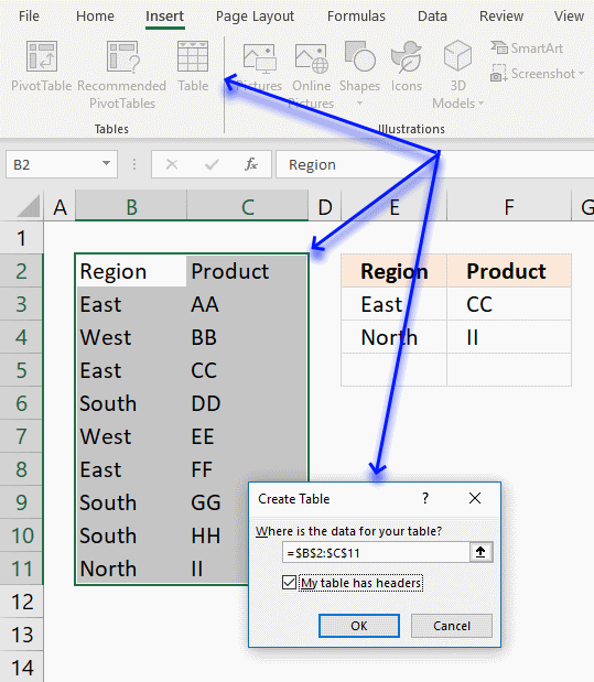
Here is how to create an Excel defined Table:
- Select cell range B2:C11.
- Go to tab "Insert" on the ribbon.
- Press with left mouse button on "Table" button.
- Press with left mouse button on the checkbox "My table has headers" if your data set has headers.
- Press with left mouse button on OK button.
The main reason I am using an Excel defined Table here is that you can use a "structured reference" which is basically a table name instead of a regular cell reference.
Relationships between categories
The first array formula returns unique distinct values in cell H2:M2 from named range Region. The second array formula in cell range H3:M7 returns coherent values from each region. All of these calculations can be hidden or placed on a calculation sheet.
Array formula in cell H2:
To enter an array formula, type the formula in a cell then press and hold CTRL + SHIFT simultaneously, now press Enter once. Release all keys.
The formula bar now shows the formula with a beginning and ending curly bracket telling you that you entered the formula successfully. Don't enter the curly brackets yourself.
Array formula in cell H3:
Copy cell H3 and paste to cell range H3:M8, if you have more categories (Regions) and Items (Products) than this example you may have to extend the formulas to a larger cell range accordingly.
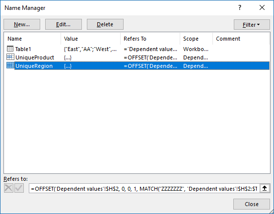
Named ranges
Now it is time to create the two last named ranges that will be used in data validation lists.
- Select cell F3, this step is very important because the named ranges contain formulas that contain relative cell ranges.
- Go to tab "Formula" on the ribbon.
- Press with left mouse button on the "Name Manager" button and a dialog box appears.
- Press with left mouse button on "New..." button.
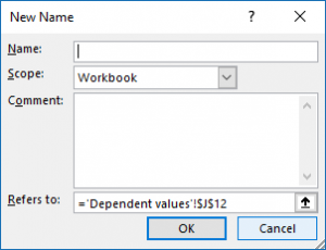
- Enter the name UniqueRegion shown below.
- Enter the formula.
- Press with left mouse button on OK button.
- Repeat step 3 to 6 with UniqueProduct
Name: UniqueRegion
Formula:
Name: UniqueProduct
Formula:
You can find an explanation to the dynamic named ranges displayed above in the article below.
Recommended articles
What is a named range? A named range is a feature in Excel that allows you to assign a specific […]
Data validation lists
The following steps shows you how to create regular drop-down lists in column E, linked to a dynamic named range UniqueRegion.
- Select cell E3
- Go to tab "Data"
- Press with left mouse button on "Data validation" button
- Select "List"
- Type =UniqueRegion

- Press with left mouse button on OK
- Copy cell E3 and paste to cells below as far as needed.
The following steps shows you how to create regular drop-down lists in column F, linked to a dynamic named range UniqueProduct.
- Select cell F3
- Go to tab "Data"
- Press with left mouse button on "Data validation" button
- Select "List"
- Type =UniqueProduct
- Press with left mouse button on OK
- Copy cell F3 and paste to cells below as far as needed.
7. Use a drop down list to filter and concatenate unique distinct values
Question: Is there a way to have a unique list generated from a list? Meaning I have a sheet that contains my data and I want to generate a drop down list based on the input from one column. Which I already have.
Once the user selects the value from the drop down, I want it to generate another unique list just in a column.
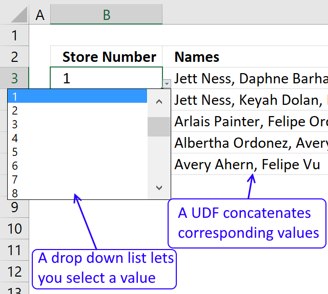
For example the sheet contains store numbers (one column) and employee names (a second column), which may be listed multiple times. I want to create the drop down for the store number and then creating a list of employee names (non-repeating) that isn't a drop down, just a standard list is say A1, A2, A3, A4, etc
Is that clear as mud?
Thanks.
Answer:

The animated image above shows drop down lists in column A and a UDF in column B, once a value has been selected in the dropdown list the UDF looks up the value in a data set and returns the corresponding values on the same rows as the matching numbers concatenated to one cell with a comma as a delimiting character.
The UDF returns a blank in column B if the cell in column A is blank.
What you will learn in this article
- Build an array formula that extracts unique distinct numbers sorted from low to high.
- How to use a named range.
- How to create a drop down list containing named range that points to numbers
- How to create a user defined function that extracts and concatenates values based on a drop down list value.
7.1 Customize worksheet "Data"

Column A contains store numbers and column B contains the corresponding name. The formula in cell E3 extracts all numbers from column A ignoring duplicates, sorted from low to high or ascending order.
Array formula in cell E3:
7.2 How to create an array formula
- Select cell E3
- Paste formula to cell
- Press and hold Ctrl + Shift simultaneously.
- Press Enter once.
- Release all keys.
The formula is now surrounded with curly brackets, they appear automatically if you did the above steps correctly. Do not enter the curly brackets yourself.
7.3 How to copy array formula
- Select cell E3
- Copy cell E3 (keyboard shortcut CTRL + c)
- Select cell range E4:E29 with you mouse.
- Paste (Keyboard shortcut: CTRL+v)
7.4 Explaining formula in cell E3
Step 1 - Ignore previously returned numbers above current cell.
The COUNTIF function lets you check which numbers have been returned above the current cell, the first argument contains an expanding cell reference that grows when you copy the cell and paste to cells below.
COUNTIF($E$1:E1, $A$2:$A$100)
becomes
COUNTIF("Unqiue store numbers",{22; 24; 9; 12; 5; 17; 22; 23; 0; 1; 14; 20; 16; 3; 25; 1; 12; 12; 20; 8; 7; 1; 2; 2; 7; 14; 4; 14; 22; 21; 8; 15; 17; 9; 12; 7; 19; 12; 7; 18; 4; 1; 14; 17; 7; 10; 16; 4; 2; 12; 19; 15; 15; 8; 3; 14; 12; 1; 5; 19; 16; 8; 15; 7; 18; 18; 2; 3; 14; 19; 9; 15; 11; 17; 23; 6; 12; 5; 5; 25; 9; 14; 25; 22; 22; 24; 2; 22; 21; 1; 20; 11; 16; 5; 5; 21; 0; 12; 1})
and returns
{0; 0; 0; 0; 0; 0; 0; 0; 0; 0; 0; 0; 0; 0; 0; 0; 0; 0; 0; 0; 0; 0; 0; 0; 0; 0; 0; 0; 0; 0; 0; 0; 0; 0; 0; 0; 0; 0; 0; 0; 0; 0; 0; 0; 0; 0; 0; 0; 0; 0; 0; 0; 0; 0; 0; 0; 0; 0; 0; 0; 0; 0; 0; 0; 0; 0; 0; 0; 0; 0; 0; 0; 0; 0; 0; 0; 0; 0; 0; 0; 0; 0; 0; 0; 0; 0; 0; 0; 0; 0; 0; 0; 0; 0; 0; 0; 0; 0; 0}
If a value is 0 (zero) in the array then the corresponding number has not yet been returned in above cells.
Step 2 - Check if value in array equals 0 (zero)
The equal sign allows you to check if a value in the array is equal to a given condition.
COUNTIF($E$1:E1, $A$2:$A$100)=0
becomes
{0; 0; 0; ... ; 0}=0
and returns
{TRUE; TRUE; TRUE; ... ; TRUE}
The array is shortened.
Step 3 - Return value from column A if value in array is TRUE
The IF function lets you return a given value if the first argument evaluates to TRUE and another value if the argument evaluates to FALSE. We are working with arrays so the position of each value is important since the corresponding value is returned.
IF(COUNTIF($E$1:E1, $A$2:$A$100)=0, $A$2:$A$100, "")
becomes
IF({TRUE; TRUE; TRUE; ... ; TRUE}, {22; 24; 9; ... ; 1}, "")
and returns
{22; 24; 9; ... ; 1}.
Step 4 - Return the smallest value in array
The SMALL function allows you to extract the k-th smallest number, however, in this case we always extract the smallest number since the COUNTIF function keeps track of previously returned numbers.
SMALL(IF(COUNTIF($E$1:E1, $A$2:$A$100)=0,$A$2:$A$100, ""), 1)
becomes
SMALL({22; 24; 9; ... ; 1}, 1)
and returns 0.
Create a named range
- Go to tab "Formulas"
- Press with left mouse button on "Name Manager" button
- Press with left mouse button on "New.."
- Type UniqueStoreNumbers
- Select cell range =Data!$E$2:$E$27 in Refers to:
- Press with left mouse button on OK!
If you know you will be adding data later on then a dynamic named range is a better choice, it grows automatically when new data is entered.
7.5 Customize worksheet: Sheet1

7.5.1 Create drop down list
- Select cell A2
- Go to tab "Data"
- Press with left mouse button on "Data validation.." button
- Go to tab "Settings"
- Select List in Allow: field
- Type in source: field: =UniqueStoreNumbers
- Press with left mouse button on OK
7.5.2 Copy drop down list and paste to cells below
- Select cell A2.
- Copy cell (CTRL + c).
- Select cell range A3:A100.
- Paste values (CTRL + v).
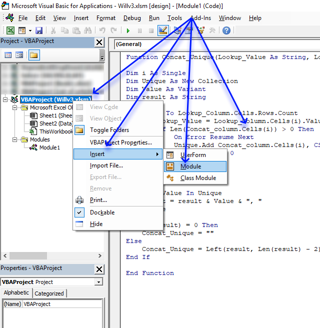
7.5.3 Add vba code to module
- Copy VBA code below.
- Press Alt+F11 to open the Visual Basic Editor.
- Press with right mouse button on on workbook in Project Explorer
- Press with mouse on Insert and then Module.
- Paste VBA code to the code module.
- Return to excel.
7.5.4 How to enter the User defined function
Formula in cell B2:
Copy cell B2 and paste to cell range B3:B8.
7.6 Vba code
'Name User defined Function and input variables
Function Concat_Unique(Lookup_Value As String, Lookup_Column As Range, Concat_column As Range)

'Dimension variables and declare data types
Dim i As Single
Dim Unique As New Collection
Dim Value As Variant
Dim result As String

'Iterate through lookup column
For i = 1 To Lookup_Column.Cells.Rows.Count

    'Check if lookup value is equal to value in lookup column
    If Lookup_Value = Lookup_Column.Cells(i).Value Then

        'Check if character length is larger than 0 (zero)
        If Len(Concat_column.Cells(i)) > 0 Then

            'Enable error handling
            On Error Resume Next

            'Add value to collection. Returns an error if there is a duplicate in the collection
            Unique.Add Concat_column.Cells(i), CStr(Concat_column.Cells(i))

            'Disable error handling
            On Error GoTo 0
        End If
    End If
Next i

'Iterate through collection
For Each Value In Unique

    'Add values in collection to a string variable with a comma as a delimiting character
    result = result & Value & ", "

'Continue with next value in collection
Next Value

'Check if variable result is empty
If Len(result) = 0 Then

    'Save a blank to variable result
    Concat_Unique = ""

'If not empty
Else

    'Remove two last characters (comma and a space character) and then return string to worksheet
    Concat_Unique = Left(result, Len(result) - 2)
End If

End Function
Dependent Drop Down Lists AddIn
Dependent drop down lists is an AddIn for Excel 2007/2010/2013 (not Mac!) that lets you easily create drop down lists (comboboxes, form controls) in Microsoft® Excel.

What are dependent drop down lists?
A dependent drop down list changes it´s values automatically depending on selected values in previous drop down lists on the same row.
The first drop down list in the picture above contains values from "Region" column. The second drop down list contains values from "Country" column and the third from City column.
Now depending on the selected value in the first drop down list, the second and third drop down lists change their values automatically.
In the picture above, the first drop down list has the value "Europe" selected, the second "France and in the third you can choose between "Lyon" or "Paris". You can see how the columns are related to each other if you examine the table above.
Features
- Utilizes a pivot table to quickly filter and sort values for maximum speed
- The drop down lists are populated using Visual Basic for Applications
- No excel formulas
- Easily copy values: Each drop down list is linked to the cell behind.
- You can create as many drop down lists you want
- You can send workbooks containing dependent drop down lists to friends, colleagues etc, as long as they can open macro-enabled workbooks.
For simplicity, your data set must be an excel table. That is easily created if you don´t know how. A vba macro is required in your workbook. The AddIn shows you how in a few simple steps.
Watch a video where I demonstrate the Add-In
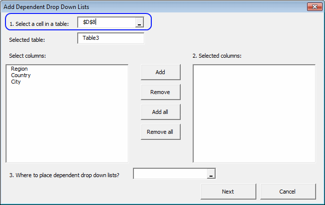
How to use the AddIn
- Go to tab "Add-Ins"
- Press with left mouse button on "Dependent Drop Down Lists AddIn" button

- Select a table


- Select desired table column headers

- Select a cell range where you want your drop down lists


- Press with left mouse button on "Next"
- Copy code to a module

- Press with left mouse button on Close

[/expand]
Purchase Dependent Drop Down Lists Add-In for Excel 2007/2010/2013 - Price $19 USD


Questions
Is there a money back guarantee?
Sure, you have un-conditional money back guarantee for 14 days.
Does it work on a Macintosh?
No
Why form controls?
A form control may have a macro assigned that runs when a new value is selected. This makes it possible to manipulate all drop down lists with a single macro.
Why a pivot table?
A pivot table filters and sorts values extremly quickly. Of course, it is possible to filter and sort values using vba but working with large data sets, a pivot table rules when it comes to speed!
Do the excel table, pivot table and the drop down lists have to be on the same sheet?
No, but they must be in the same workbook.
Can I create dropdown lists on multiple rows?
Yes, insert dropdown lists on multiple rows using the add-in. However, you can´t copy and paste the dropdown lists yourself, they have unique names.
What customizations can I do with a combobox (form control)?
You can change the number of drop down lines, 3d effects and link each drop down list to a single cell.
Can I hide the pivot table sheet?
Yes! Press with right mouse button on on the sheet and press with left mouse button on "Hide"
Can I change the order of drop down lists?
Yes, rearrange the table columns and then use the AddIn to create drop down lists.
If I construct a UI using the AddIn, then will anyone be able to use those on their own computers without adding the AddIn themselves?
Yes, they will be able to use the drop down lists.
If so, then would they just need to enable macros?
Yes, that is correct.
Testimonials
The add-in makes dependent drop-down lists easy and flexible to implement in Excel. It fills a vital missing gap in Excel's functionality, because the drop-downs feed data into the underlying cells that they float over. It is simple and straightforward to integrate them with your own spreadsheets. Excellent support from the developer.
Isn’t it surprising that making dependent drop-down lists is still so difficult in Excel? The Dependent Drop Down Lists add-in makes it much simpler. Plus, they have excellent customer support if you get stuck.
How the Purchase Process Works?
- Payment is accepted via PayPal.
- After you finish payment, you are redirected to the get page. You will also receive an email with the get link.
- You have five attempts to get the file.
- The get link will expire in 120 hours (5 days).
If you can´t geting the file, contact me.
Dependent drop down lists category
More than 1300 Excel formulasExcel categories
188 Responses to “Create dependent drop down lists containing unique distinct values”
How to comment
How to add a formula to your comment
<code>Insert your formula here.</code>
Convert less than and larger than signs
Use html character entities instead of less than and larger than signs.
< becomes < and > becomes >
How to add VBA code to your comment
[vb 1="vbnet" language=","]
Put your VBA code here.
[/vb]
How to add a picture to your comment:
Upload picture to postimage.org or imgur
Paste image link to your comment.
finally! :)
but attached file is empty?
david,
A new excel file is attached!
Thanks for commenting!
works great and marvellous work!
thansk! ;)
this process works to perfection! thanks so much for posting. now if i only knew how to apply these dropdown selections to a filter, i'd be set.
Josh,
read this post: Apply dependent combo box selections to a filter in excel 2007
I just came across your site as I was looking to do this very thing, (with a slight twist). I am setting up a sheet where the same type of dynamic lists were needed for multiple entries. I.e. I needed to be able to make an entry in one column from a drop down list and have a dependant list on the same line in the next column, THEN have the dependant list update based on the new entry on the next line. Using you list formulas and adding a very slight modification I am able to implement the dynamic drops lists I needed. Thanks very much!
how would i make this also be alphabetical?
Fantastic!
jon,
Sheet2:
Array formula in cell A2:
=INDEX(order, MATCH(SMALL(IF(COUNTIF($A$1:A1, order)=0, COUNTIF(order, "<"&order), ""), 1), IF(COUNTIF($A$1:A1, order)=0, COUNTIF(order, "<"&order), ""), 0)) + CTRL + SHIFT + ENTER. Copy cell A2 and paste it down. Array formula in cell B2: =INDEX(product, MATCH(SMALL(IF((COUNTIF($C$1:C1, product)+(order<>Sheet1!$D$2))=0, COUNTIF(product, "<"&product), ""), 1), IF((COUNTIF($C$1:C1, product)+(order<>Sheet1!$D$2))=0, COUNTIF(product, "<"&product), ""), 0)) + CTRL + SHIFT + ENTER. Copy cell B2 and paste it down as far as needed.
Hi,
I tried to use this formula, but the unique values some how are giving duplicate values for me.
Sharmila,
Did you change the relative and absolute cell references (bolded) in both formulas?
=INDEX(order,MATCH(0,COUNTIF($A$1:A1,order),0))
=INDEX(product, MATCH(0, COUNTIF($B$1:B1, product)+(order<>Sheet1!$D$2), 0))
Oscar,
thanks for the reply. i entered the formula into A2 and that worked but the formula for B2 didnt work. i was wondering maybe it was becasue the formula referenced "$c$1:c1" so i changed it to reference "$b$1:b1" since i was entering the formula into B2 but that didnt work either. any advice?
thanks in advance.
figured it out. it had to do with the $C$1:C1 as i guessed as well as all the spaces in the formula. i took out the spaces and it worked perfect.
thanks! great formula!
I am happy you figured it out!
Hi,
I have a question, how can i use these list for multiple rows?
I would like to use these lists for multiple rows and let people enter detailed records.
I have no words to thank you
The answer to Sharmilas question can be found here: Create dependent drop down lists containing unique distinct values in multiple rows
Hi,
Would there be any changes in the formula if Product in the first column and Order#ID in the second column?
Thanks
sanlen
sanlen,
No, the formulas work with both numbers or text.
Hey, thanks for this wonderful information.
I need one more addition. How can i make it generic, instead of copying the cell & pasting it all the way down?
Suraj,
I am not sure I understand.
Try this formula in A2 and cells down:
=INDEX(order, SMALL(IF(MATCH(order, order, 0)=(ROW(order)-MIN(ROW(order))+1), ROW(order)-MIN(ROW(order))+1), ROW()-1)) + CTRL + SHIFT + ENTER
Array formula in B2 and cells down:
=INDEX(product, SMALL(IF(IF(ISERROR(MATCH(IF(order=Sheet1!$D$2, product, FALSE), IF(order=Sheet1!$D$2, product, ""), 0)), "", MATCH(IF(order=Sheet1!$D$2, product, FALSE), IF(order=Sheet1!$D$2, product, ""), 0))=(ROW(product)-MIN(ROW(product))+1), ROW(product)-MIN(ROW(product))+1), ROW()-1)) + CTRL + SHIFT + ENTER
Oscar,
I am trying to do this on multiple columns?
Crop Select SF/ST Qty
ARA PLANTS UNTREATED 1 PLANT
ARA SEEDS STANDARD TREATMENT 1 SDS
ARA SEEDS UNTREATED 10 SDS
ARA 100 SDS
ASA 1 SDS
ASA 10 SDS
ASA 50 SDS
BDB SEEDS ITALIAN TREATMENT 20 KG
BDB SEEDS LORSB./THIR/APR. 25 KG
BDB SEEDS STANDARD TREATMENT 25 SDS
BDB SEEDS UNTREATED 5 KG
BDB 5 SDS
BNC SEEDS ITALIAN TREATMENT 0,100 KG
BNC SEEDS LORSB./THIR/APR. 0,250 KG
BNC SEEDS STANDARD TREATMEN 1 KG
BNC SEEDS UNTREATED 1 SDS
BNC 250 SDS
The column 2 and 3 are independant of each other but dependent on the first column
Deb,
I think you need to read this article: https://www.get-digital-help.com/create-dependent-drop-down-lists-containing-unique-distinct-values-in-multiple-rows/
You can then apply dependent drop down lists on multiple rows.
Oscar,
I meant to say:
Instead of copying cell A2 & B2 all the way down in Sheet2, is there a generic way of doing that? Can the formula be automated, so as to avoid #N/A in the cells on Sheet2?
Suraj,
#N/A´s are avoided by using a dynamic named range and are not displayed in any of the drop down lists.
=OFFSET(Sheet2!$A$2, 0, 0, COUNT(IF(Sheet2!$A$2:$A$1000="", "", 1)), 1).
IFERROR() function prevents error messages in cells.
Oscar,
Thanks a lot. I would rather hide the calculation sheet(Sheet2), than to try and hide/manipulate the #N/A values. :-)
Anyways, Great Work. Keep it up!
It helped me a lot.
Hi,
I am trying to filter values in a drop down menu based on the values entered in the previous drop down menu.
eg: i have values 1,2,3,4,etc in drop down cell 1.
i want to filter values in drop down cell which contains 111,222,22,333,444,etc..
If I enter 2 in cell 1 then the second cell should filter values and show only 222 and 22...
Thanks in advance...
Amit
Amit,
Instead of creating unique distinct values you need to filter values.
try formula:
=INDEX(array, SMALL(IF(ISERROR(SEARCH($H$3, array)), "", ROW(array)-MIN(ROW(array))+1), ROW(A1))) + CTRL + SHIFT + ENTER
Adjust cell references and named ranges to your sheet.
Its working very well...........but i want it like this
press with left mouse button on an alphabet its should move to the corresponding list
Its working very well...........but i want it like this
on press with left mouse button on an alphabet its should move to the corresponding list
if any alphabet is entered it should get all list corresponding to that alphabet
Shikhar,
can you elaborate? Can you provide an example?
For Eg:-i have created a sheet named list
it has 5 columns
1st column contains:4 project types development,documentation,maintainence,lotus notes
2nd column contains:all the development projects
3rd column contains:-all the documentation projects
4th column contains:-maintainence projects
5th column contains:-lotus notes projects
I have put a validation on some other sheets so that according to the project types the projects are coming and the user can select his particular choice.
Till here its working fine
But if a user is pressing any alphabet say "A" I want is that the control should go to the project starting with A........
@ oscar thanks for replying me and if possible get some alternative for this......
shikhar,
Predictive text is possible in combo boxes (ActiveX) with some programming.
See Contextures: Excel Data Validation Combo box using Named Ranges
Hi Oscar,
Thank you for the wonderful solution.
I am attempting to recreate what you have done in Excel 2007. I seem to be having issues with the following line:
=INDEX(order,MATCH(0,COUNTIF($A$1:A1,order),0)) + CTRL + SHIFT + ENTER
If I open your file in compatibility mode then the following formula is found in its place
{=INDEX(order,MATCH(0,COUNTIF($A$1:A1,order),0)) }
but if I attempt to select the formula then the brackets automatically are removed and I get an error message in the cell.
Any insigh is greatly appreciated.
Thank you in advance for your assistance.
Roy
Roy Shore,
The brackets indicate array formula. Press and hold CTRL + SHIFT and then press Enter to create an array formula.
Read this: Introduction to Array Formulas
Thanks for commenting!
Oscar........ thanks a lot for the solution this is Exactly what i wanted.............
I currently am using a Mac with Excel 2008 and can't seem to locate the "Formulas tab" and "Name Manager" to create a dynamic named range like you did. Can you help me? Just learning...
Darold,
I wish I could help you! But I don´t know.
Found it! It is under the "Insert" tab, then "Name", then "Define".
Thanks!
What is the formula if there is a third column of data?
Patrick,
Get the example workbook with a third column of data
unique-distinct-dependent-lists1 three columns.xls
(Excel 97-2003 Workbook *.xls)
Oscar, thank you for this information. This post is a great help. I have this working right now with 6 drop downs/lists. I wanted to see if you possibly know of a way to see additional information in drop down #4 if there are no selections in drop down #2 and #3. Currently, I have hemisphere in drop down 1, Sector in drop down 2, Region in drop down 3, and Area is drop down 4. If I select a value in drop down #1 (Hemisphere), I would like to see what areas I can filter on in drop down #4 without having to select values in drop down 2 and 3. Is there a way to make that work?
Josh,
Great question!
Read this: Dependent drop down lists – Enable/Disable selection filter
Outstanding, this works beautifully. Thanks for sharing your expertise.
Hello,
Great work so far but I was wondering if it could do something else...?
If I start off with all the down lists as empty and then, say, select keyboard as the product it successfully shows only US and Europe as the options - but shows both order ID, when it can only come from 1020.
Is it possible for the list to work both ways? Also, what if you were to select Asia and Graphics card - could it automatically fill in 1020 (the auto filling is more of a nice feature than necessary..:))
Any help or advice would be greatly appreciated, thanks!
Charlie,
Question 1:
Get the example file
dependent-drop-down-lists-selection-filter_charlie.xls
Question 2:
I think autofilling is possible with combo boxes:
Apply dependent combo box selections to a filter in excel 2007
Thanks very much!!!
Oscar, This post satisfied an exact requirement of mine and has been very helpful indeed. However, if I select my way thru the drop down lists too quickly in Excel 2010 it causes it to crash. If I wait for the field to populate each time I make a selection it works fine but if I hurry thru it then it always crashes. Tried the same file in Excel 2007 and no problem at all. Have you experienced this problem with 2010?
Paul,
I have to admit, I have not yet bought excel 2010.
How can additional colums with more criteria be added to the exsisting three columns? Can drop boxes be added to multiple rows, such as in an Invoice? I seen your example "Create dependent drop down lists containing unique distict values in multiple rows" but how can those formulas be combined with the formulas in this example?
Can a fourth and five column be added?
Can I add 3rd, fourth and fifth column of criteria such as size and color?
Oscar, I have a problem. I am building this form for my startup company in EXCEL 2003. I have one column with dropdown list with the parts I am selling. In the other column I want the prices to be automatically added to the cell when I select the part from the dropdown. How do I do that?
Thanks in advance
Many thanks to you. That's actually one of the best tips I've ever received for Excel. Works like a charme, even when going for more sheets involved (maybe more tricky then, however, still working with some modifications).
hi Oscar,
would know how this can be done using Form Control?
panda,
See this blog post:
Apply dependent combo box selections to a filter in excel 2007
Dear Sir,
I am very much impressed with use these formulas.
With Regards
[...] -- Dependent Lists zie Excel Data Validation -- Dependent Lists With INDEX voor unieke waardes zie Create dependent drop down lists containing unique distinct values in excel | Get Digital Help ik heb dependent data validation nooit dieper zien gaan dan 3 nivo's als je het met formules wil [...]
hi there - is it just me !! can any one explain why when i type in the bing browser "www.get-digital-help.com" i get a different site yet whe i type it in google its ok? could this be a bug in my system or is any one else having same probs ?
alf saden
Oscar, thank you very much for the help. You have saved me many hours and taught me a lot.
I am having the same problem that Paul is having with 2010. If I try to select the drop down menu very fast in 2010, Excel crashes. In 2007, the "waiting" symbol on the mouse appears for maybe half a second, and then everything is fine. Anyone have any ideas on how to help.
Hi Oscar,
Thanks for the great work you are doing.
I am not an expert, and I was wondering if there is any way that you can do and publish the same for 7 columns.
Also, is the excel addin that you have created available for free somewhere?
Thanks a lot for answering my question.
Nilhan
Hello All,
My Question,
I need to create another dependent drop down list based on the first one list? If i change the first list "A" so i will get the results on "B" and "C"
here the link for MREXCEL forum the file is there.
https://www.mrexcel.com/forum/showthread.php?t=610600
please advice.
Said,
If I am not mistaking, I think my answer to Dan answers your question.
Oscar, thank you for the help. still the problem is not solved yet. would you please have a look for the excel sheet see if you can do it there? i have done the first dependent list but still i can't do the second! can you please do it for me??
thank you again.
Said,
Contact form
Oscar instead of using "ZZZZZ", use a "Ω" to the same effect. Applicable only for finding the last Text.
chrisham,
thanks!
Hi Oscar,
Thanks for this useful tip.
I have a query for Excel 2007.
I made a drop down list which includes 2 departments. Finance Dept and HR Dept.
In the dependent column, I mentioned the designations within the above 2 departments.
When I select Finance Department, the dependent list shows me the designations in that department and I select one designation in it e.g Senior Accoutant.
however, when i select HR deparment,it continues to show Senior accoutant in the dependent list. I want it to be updated itself and show the top most designation in the HR dependent list.
How do i do that ?
Thanks
Haroun,
I believe this post answers your question:
Apply dependent combo box selections to a filter in excel 2007
Hi,
I have followed the instructions here but have a question. I have a list of Categories and associated Subcategories.
I want to create the dependant drop downs for use on a form people will fill out. On the form they will select "category" via the first drop down and then select an allowed 'subcategory' via the dependant drop down.
It seems when you create the dependant drop down in the last step of your instructions, you are linking it to the first drop down (in your example uniqueorder).
In teh form I am trying to build I want to have several rows that allow people to utilize the drop downs.
I haev tried editing the conditional dropdown to reflect the new location of the first drop down, but this does not seem to work.
Any ideas?
Thanks!
I am having a small issue. This seems to work almost perfectly. They only thing that I can't seem to understand is why it is not returning all the sub categories that I have once we get past a certain number of main categories.
I have a 3 level of categories
Level 1, Level 2, Level 3. Level 1 has 100 entries but when I select the last category (which starts at row #93 it only return the first 2 sub categories when there are actually 9
Any Ideas
Thanks I figured this out. My named ranges were incorrectly configured.
Pierre Letourneau,
I am happy you figured it out!
Vince,
I don´t know how to create three or more dependent drop down lists on multiple rows using array formulas.
VBA solution: Create dependent drop down lists containing unique distinct values in multiple rows
If you are looking for two dependent drop down lists in multiple rows: Dependent data validation lists in multiple rows
Tks very much for yr tip.
but when I've Created a unique distinct list from column A.
type =INDEX(order,MATCH(0,COUNTIF($A$1:A1,order),0))to cell A2
result N/A
what wrong?
tks
nam,
Array formula in cell A2 (not A1):
Why did you choose 'Dependent values'!$D13 for the UniqueProduct formula?
Hey, there. This worked like a dream. Exactly what I wanted. So, I have a row with 3 drop downs, with the 2nd cell dependant on the first, and the 3rd being dependant on the previous 2. How do I duplicate this onto another row without having to create another data/list sheet and calculation sheet for every duplicate row I want to make?
Dear Mr. Oscar
thanks very much
it works
Very clear and helpful. I echo Sharmila's post. Can't thank enough.
Sandi B,
I am happy you like it! There is an alternative version with no vba:
Dependent data validation lists in multiple rows
Paulo,
You found an error, I have uploaded a new file and made some corrections to this post.
Thanks for bringing this to my attention!
Oscar,
Thank you for such an informative discussion on this topic. I have a question on the drop-down lists. Once the coding is done as shown and I tried it on two sets of data, the user cannot input a value from his own. He is only restricted to those values. What if I want to have a drop-down list and as well the user can input his own value i.e., a custom value.
I am trying to make a calculator where the bolt sizes can be selected from a drop-down list in a cell but also one can input his own bolt size in the same cell. What changes would I need to make to the code?
Thanks in advance.
Question: Is there a way to have a unique list generated from a list? Meaning I have a sheet that contains my data and I want to generate a drop down list based on the input from one column. Which I already have.
Once the user selects the value from the drop down, I want it to generate another unique list just in a column.
For example: the sheet contains store numbers (one column) and employee names (a second column), which may be listed multiple times. I want to create the drop down for the store number and then creating a list of employee names (non-repeating) that isnt a drop down, just a standard list is say A1,A2,A3,A4,etc
Is that clear as mud?
Thanks.
Will,
Yes, I think I understand. I have to use an udf to concatenate values.
Check out this file:
Will.xlsm
Hi Oscar,
What about my data list of the Product have duplicated value and I only want to show unique value?
=INDEX(Product, SMALL(IF(G$1=Region, MATCH(ROW(Region), ROW(Region))), ROW(A1)))
Also, how can I make a list to match 2 value?
Here is my data sample ( My lst is huge!)
Division Dept Line Subline
Women D121 Tops T-shirts
Women D121 Bottom Plants
Women D123 Tops Jacket
Women D121 Tops Jacket
Mens D124 Bottom Plants
Mens D124 Bottom Underwear
Mens D125 Bottom T-shirts
..............................
Before, I use vba to write the data validation. However as the list is too large. The excel sometimes become no responding and take times to write the unique list.
Thank you!!!!!
Penny,
Before, I use vba to write the data validation. However as the list is too large. The excel sometimes become no responding and take times to write the unique list.
I don´t think a formula is faster for filtering unique distinct values. I would suggest using vba and pivot table:
Excel vba: Populate a combobox with values from a pivot table
Change pivot table data source using a drop down list
Dependent Drop Down Lists AddIn
I am trying to create an estimating form that will calculate a total cost based of the values given. I have a drop down list, and i want it to produce a $ value for each item in a different cell. My goal is to create a form that will calculate total values.
The dependent drop down list macro works like a beauty when working with small quantities of data :-)
However, my plan was to use it for the user to specify valid product configurations when specifying sales forecasts (about 1.000 - 2.000 product forecast lines). The product structure include 3 levels;
1) Product Line; (Currently 3 product lines)
2) Product Series; Within each Product Line there are a number for Product Series (about 10+- Product Series within each Product Line
3) Product Model; There are multiple Product Models (8 - 20 Models pr Series) within each Product Series.
A typical forecast entry line looks like this;
Customer / Project, Product Line, Product Series (within p.line), Product Model (within Line, and Series) [I use dependent drop down lists for this] Multiple lookups from a product table looking up selected product attributes including price etc.
As stated above, it works like a beauty with a 10 - 30 lines, it gets very slow when getting close to 100 and unacceptable (and I have experienced even full breakdown) after 150 -- fare from target 1-2.000 lines.
Please advice.
Dag
Dag,
Perhaps you have more cpu intense formulas in your sheet?
Hi Oscar,
I'm trying to use the above information (very helpful by the way) to create an order form for products; whereby a customer can select the type/category, and then subsequent information after that. The problem is that I cannot get my head around how to arrange the drop-down boxes & the information.
I would like to hide the product information in a sheet, and have the order form in another.
I understand the above example is to be used to retrieve entered information for record keeping - is there any way I can create a form?
Regards.
Callum.
Hi Oscar.
Great site! I've worked with this today and as long as there is more than one entry in a list then the dependant list works well.
I have 3 columns with 2 dependant lists
Column 1 = Category 1
Column 2 = Category 2 Which can have from 1 to 25 items depending on the selection in Category 1
Column 3 = Category 3 Which can have from 1 to 25 items depending on the selection in Category 2
If category 2 has only one item then only errors are displayed in Category 3 even if there are values.
I am filtering these lists from an Excel Table
I've looked at the formulae, but I can't work out which bit to amend. I think that the problem lies with $A$1:A1, but I don't really understand the syntax. Could you explain further please?
Kind regards
Philip Smith,
I recreated your setup with the attached file, using one item in category two. It seems to work.
$A$1:A1 is a cell range that automatically expands when you copy the cell (not the formula). $A$1 is an absolute cell reference, it does not change. A1 is a relative cell reference, it changes.
Copying the cell to the next cell below changes the formula to $A$1:A2.
[...] have the information you want. I can't remember exactly where I found the advice, but this link https://www.get-digital-help.com/2010...lues-in-excel/ should help. Your requirements are entirely achievable. Regards [...]
Hi,
I had a question. I have a excel costing sheet. What it is is a pull down menu with options to build a trailer.
So one pull down menu is tires. Then i pull down and it has a bunch of different tire options. My question is how do i get the price to change when i select different tires?
There are 3 tires. Goodyear is 500.00 RM is 400 and DL is 800.00
so i go to the pull down menu and choose a tire then i need the correct price to go in the price box beside that. I have aformula to do this but it's so long and i think it can be alot easier.
Right now this is the formula:
=IF(A51="X",VLOOKUP(B51,Sheet1!$A$2:$B$12001,2,FALSE),"-")
BUT what it does is look up on one sheet who gets its information from another sheet who gets its information from another sheet. So there are all these sheets and im pretty sure i don't need them all. It's just making this spreadsheet very large and very slow!
Please help if you can
Aynsley,
Your formula seems to be fine.
yes, i know my formula is fine but i think it requires way too much work to do something that seems fairly simple.
it takes it's information from the options work sheet. which looks the price up on the price worksheet which looks it up on another work sheet to get the inforamtion.
it just seems like something could be cut somewhere.
I have a list where not all the cells are populated. Tried the method above but the unique list appears to be incomplete (e.g missing values). Any way to make this work for me. Really appreciate your assistance.
Example:
List = A1:A20
Populated = A2:A10,A15:A17
Not Populated = A1,A11:A14,A18:A20
Ahmad,
Did you adjust the cell reference (bolded)?
Array formula in cell A2, sheet 2:
=INDEX(order,MATCH(0,COUNTIF($A$1:A1,order),0)
[...] into a unique list that is organized. I've used the index function (similar to what is used in Create dependent drop down lists containing unique distinct values in excel | Get Digital Help - Mic... ) to do it, however, because I'm using 1,000+ lines about 50+ uniques in a single column, it tends [...]
Thank you Oscar!
exist too solution for google spreadsheet? everything works, but I have problem only with the application to next rows.
Sievert,
I have problem only with the application to next rows.
Can you explain in greater detail?
Please Oscar, look at the link - https://www.mrexcel.com/forum/excel-questions/669408-dependent-drop-down-lists-google-spreedsheet-values-multiple-rows.html .
I tried to more explain.. Thank you
Sievert,
Only one thing doesn't work Application function to the next rows.. I tried use timestamp, but without successful, maybe I used wrong it.
I still don´t understand and I don´t know much about google spreadsheets.
Sorry, my mistake..
When you open spreedsheet :
https://docs.google.com/a/linksoft.cz/spreadsheet/ccc?key=0Asiaoa2t4PpGdGJDWk5wSE43LVdyTXJHU3R0SHdkY0E#gid=1
look at the row 2, dependent list works correctly, when you look at the row 3, dependent list doesn´t work.. because now you can see values B1 and B2... but still you can see values from the previous row 2... so function works only for second row and the multiple rows doesn´t work :(
[...] drop down lists containing unique distinct values in spreedsheet according to the instructions ( Create dependent drop down lists containing unique distinct values in excel | Get Digital Help - Mic... ) , everything works like in excel. Only one thing doesn't work Application function to the next [...]
[...] what was selected first: picture hosting So I got that working using instructions found here: Create dependent drop down lists containing unique distinct values in excel | Get Digital Help - Mic... The method shown there does work, but only for that particular row. If I copy it down, it won't [...]
This is exactly what I was looking for. I am just trying to understand how it works. I have understood what is going on up to the point where you use the function IF(Sheet2!$B$2:$B$1000="", "", 1), I can see that it returns a 1 into an array for cells that are neither blank nor #N/A, but why does the test ="","" do this.
Matthew Gavanda,
why does the test ="","" do this
Great question! I don´t know why it does that.
COUNT(IF(Sheet2!$A$2:$A$1000="", "", 1)) counts cells that are neither blank nor #N/A
COUNTA(Sheet2!$A$2:$A$1000) counts ALL cells except blanks
Hi Oscar,
I am following your steps and I am now on "Create a unique distinct list from column A" topic. When I do the CTRL + SHIFT + ENTER in the cell with the formula "=INDEX(order,MATCH(0,COUNTIF($A$1:A1,order),0))", Excel opens a Window with the "Update Values: Sheet1" title. When I close that window, the function returns the value #VALUE!
Do you know what I could be doing wrong?
Thank you and regards.
Rejane
order - is a named range. If that named range is not in your spreadsheet, the formula won´t work.
Open the attached file in this post and check it out.
Hi Oscar,
This formula works fine with small tables and where data in a column are of the same type (either numbers or text).
Can you suggest a solution for the kind of cases I mention above, except using VBA?
Thanks,
Eduard
Eduard,
Large data sets?
No.
where data in a column are of the same type (either numbers or text)
As far as I know, the formula extracts both numbers and texts combined? Can you provide an example?
Why you used "zzzzzz" what it will do. can we add "sukhdev" in place of "zzzzzz". will it work or not??? kindly let me know.
Sukhdev,
MATCH("ZZZZZZZZ", 'Dependent values'!$A:$A)-1 returns the last cell row containing a text string. You could use this value: ÿ instead to make sure all text strings are matched.
What should we use for Numbers (code) and text both. Please help me.
Sukhdev,
Try this:
=MAX(MATCH("ÿ",'Dependent values'!$A:$A),MATCH(9E+307,'Dependent values'!$A:$A))-1
Hi Oscar Thanks for reply
I tried the same in Name manager but did get success. I Used below formula in Name Manager;
=MAX(MATCH("y",Sheet1!$A:$A),MATCH(9E+307,Sheet1!$A:$A))-1 (for Column A)
=MAX(MATCH("y",Sheet1!$B:$B),MATCH(9E+307,Sheet1!$B:$B))-1 (for Column B)
and My data is below.
Material Group Material Name
1156 Mouse Optical Neo Usb
1187 UPS Black Armour 725
1187 UPS Black Armour 725
1112 COMPUTER M/M SPEAKER BEATS IT-1875 SUF R
1111 Computer Cabinet P4 Entizer W Smps & Usb
1111 Computer Cabinet P4 Supernova RB w smps
1111 Computer Cabinet P4 Orion RB w smps & us
1111 Computer Cabinet P4 Empower- R w smps &
1196 Data Card Speed-3Gv 7.2”(Modem)
1112 Computer Multimedia Speaker IT 2000 Sb J
Sukhdev,
No, I just pointed out the part of the formula that returned the error. Here is the whole formula:
=OFFSET(Sheet1!$A$2, 0, 0, MAX(MATCH("ÿ",Sheet1!$A:$A),MATCH(9E+307,Sheet1!$A:$A))-1)
See this file:
Sukhdev.xlsx
Hi Oscar,
Above mentioned Formula is working perfectly. Thanks a lot for helping me.
Thanks,
Best Regards,
Sukhdev
Sukhdev,
I am happy you got it working!
Hi Oscar
I have two columns Mcode and Mname and I wish to make dynamic drop down of unique Mcode. If I select One M code, all the Mname including duplicate under that mcode should reflect. My data is very huge so I want to create it dynamically. Please help me.
Thanks,
Regards
Sukhdev
Hey Oscar,
When I select my combo box to choose a value, the #N/A is there mutiple time. Maybe i did a step wrong. You have any idea?
Thanks !
I forgot I had another question XD. In your example, I understand that you can only have one combox box, but I want a column full of combobox and on the second column the combobox filter with the value select in the combobox in the first column of the same row.
Sr for my bad english, hope you understand!
Max
I find in the comment another example for what im looking for. But I still have my first problem with the #N/A
Max,
Hard to say, upload an example file.
Hi Oscar
Do you have a tutorial or example to do this exact same thing but using VBA?
Mike
Mike,
Sorry no.
Hello,
Maybe this is a silly question, but i have been trying to put the Dropdown lists on Sheet1 in Sheet3. When i do that i update the 2nd in sheet 2 to sheet 3 ( =INDEX(product, MATCH(0, COUNTIF($B$1:B1, product)+(orderSheet3!$D$2), 0))" + CTRL + SHIFT + ENTER) But i keep getting NV# is there something im missing?
Best regards,
Miguel Araque
I was just able to make it work !,
really good website!!
Regards
VBA Example ?
You are a genius I fan you
I want to be like you
can You OPEN and LOCK writing in columns and rows by ( DATA VALIDATION )
How To Lock Or Protect Cell Using Data Validation?
Excellent work. thanks for sharing.
If we dont want to use array fomular
maybe this is a choice
INDEX(order,MATCH(0,INDEX(COUNTIF($A$1:A1,order),),0))-->enter only
Dear sir, i need ur urgent help,
how i can use this dependent drop code in vba form of combobox.
please send me module code of that.
THanks
Sir i need it very urgent
Thank you for the wonderful tips!
I tried to edit your example with no luck...
in sheet 1, i have for example these:
A2: John, B2: Supermarket shoes
A3: John, B3: Bowling
A4: Maria, B4: Groceries
A5: Maria, B5: School
etc.
I use my own values, but the in Sheet 2, in column B i get for all values #N/A...
What exactly am i doing wrong?
Thanks again for your lovely work!
Haris Eliades,
You are right, you get #N/A when you use your values in my example.
Try changing the value in the drop down list in cell D2, sheet1 and the array formula in column B, sheet2 returns values again.
The array formula in column B, sheet2 returned #N/A because the value in cell D2, sheet1 (1010) was not found in column A, sheet2.
Why you used 'Dependent values' what it will do. can we add delete this, will it work or not??? kindly let me know.
I don't want to use 'Dependent values'! Words in formula. But I can't. We don't use the another sheet, so why we use to urgency "!" sembol with sheet name?
I can't understand why we are matching with zzzzzzzz. I don't want to use match. Could you do this example with vlookup please. Thank you.
Hi Oscar,
The dependent drop down list is perfect for a race report sheet I am developing for my sailing club (see website link). I want to be able to have the user select the race date (equivalent to the order in your example), and then select the race name (equivalent to the product). Our race calendar is typically two races per day, with a results report to be generated for each race.
I originally had my race calendar table formatted as a table, which meant when creating the first dynamic named range, Excel was changing the range in the formula to the table name (e.g. RaceDetails[@Date]). When I converted the table back to a normal range, the error was removed. Is there an adjustment to the formulas above that would allow the same result using a table range?
I'll also note that if the values in the original list contain formulas, the unique list also won't work correctly as Excel thinks each value is unique - overcome by copy and paste values into that range.
Cheers!
Mark Graveson,
Is there an adjustment to the formulas above that would allow the same result using a table range?
I have created an excel defined table and changed formulas, get file:
unique-distinct-dependent-lists1-three-columns.xlsx
Thank you for providing this! This is awesome. I did run into an issue though which I thought you might be able to help.
Whenever I save the workbook and reopen, the drop down only disaplays first two items. All the formulas are there, and I have to go into the Data Validation for each drop down and (without doing anything) just save it to re-enable the drop down.
I dug through google and didn't find much except that there is a known bug(?) which Microsoft is releasing a fix. Have you run into this issue? I do have rather large drop down (about 380) - could that be an issue?
Thank you very much for all your help!
Please disregard above question. I used the Defined Names, and the problem is resolved. Thank you again!
WJ,
Thank you for posting the solution!
Thanks so much for this-- it's been really helpful and worked perfectly for my lists with straight text entered.
I was also hoping to do the same with a list where cell values are based on CONCATENATE (from three other cells, two with names and one with a date in order to generate a unique name). I'm assuming that the above method doesn't deal with cells with forumulae (I'm returning a list of blank cells).
Is there any way for me to create an alphebetized list based on the values of these cells?
Hi there,
Kindly help me to get rid of few iss
I want to two simple dropdown list join but i cannot,
Suppose,
1st drop down list cell(A2) and second (B2)
A2=List(Samsung,Nokia)
B2=(List of samsung and list of nokia mobile name)
When select(A2) from dropdown list samsung after that B2 Show Relavent Samusumg mobile list,as same as Nokia..
So how can i join it....
Plz help me..
hi Oscar,
how can i store multiple drop down menu results onto a separate spreed sheet and keep adding to it
scott,
Can you explain in greater detail or provide an example workbook?
Hi Oscar,
I have created 2 separate wook books, one containing the lists and the other containing the categories containing the lists in the drop down format. when you select the chosen item from the drop down menu I would like to be able to press on a submit function and store the results from several lists onto a separate work book with the ability to reset and continue adding more results
thanks
Scott
[…] Perhaps there is a better solution, but if sorting the data is not an option, you may need to create a 2nd, automatically updated list, based on the first one - that also automatically sorts alphabetically. See example given in the link below Create a drop down list containing alphabetically sorted values in excel | Get Digital Help - Micros… […]
I am having trouble making the code reference different cells. My lists are not in column A and do not start at Row 1. What values in the code do I change to reference different cells?
Sometime when I paste the code for your saple to my new file, it will not function. Do you have to turn on or enable something, or is there a glitch in MS Excel program.
Need help with data similar to file Sukhdev.xlsx. Three dependent columns; first to have equipment type, second to have equipment brand and third to have the equipment model. I'm thinking I should have 2 sets of caluclation sheets similar to the one in tutorial. Is there an easier way?
Liju A,
I am not sure how, if you want to use array formulas.
My Dependent drop down list Add-In handles more than 2 columns easily.
or check out: https://www.contextures.com/xlDataVal13.html
I think this formula is really cool. I used it in my excel tool and works great.
Does this not work for lists with both alphabets and numbers?
Seems to only work for lists that are either all words or all numbers.
Hi Oscar,
Very useful indeed! thanks so much! I need it to work for 4 not 3 columns of data. Would it be possible to post an example file for this?
Many thanks
Rob
Thank you very much. So clear and very well described. Hours saved.Great help.
first list AA, BB, CC
second list under AA - 11,22,33
under BB - 44, 55 etc
I have two column ... first column contains a list of AA,BB,CC
and in the next column it should return another list based on selection in the first column. for example if i select AA in the next column it should return another list with 11,22,33
is this posible???
hello Oscar my question is on the example you made in Step number 8 , where you have a drop down menu in the bottom for anyone to choose the region, how can I make the drop down in the left to control the other cells in the same row , for example if I choose South America in region in that drop down menu, immediately the column C and D will auto populate giving me Brazil and Sao Paulo, without me having to go and press with left mouse button on the drop down menu and choose between the options one by one?
thanks in advance
john
Oscar,
superb implementation - still trying to understand it completely.
I am just using the Create a dynamic named range/Create a unique distinct list from column A/Create a dynamic named range to get unique distinct list components.
but I have 1 difference: my equivalent of col A and 'order' is implemented in an excel 'table'. it works fine. I can add/delete rows to the 'table' and it expands/contracts as expected.
however, 'uniqueorder', implemented as you describe, works just 1x. if I add/delete rows in 'order', in the excel 'table', then the worksheet with 'uniqueorder' does NOT expand/contract similarly.
is it possible that defining 'order'/'uniqueorder' to the name manager using the OFFSET function is in conflict with the excel concept of a 'table'?
anyway, thanks for getting me this far in my learning curve.
ron
ps: just 1 last question 'order'/'uniqueorder' start in row 2. now, defining the distinct list using the index function with COUNTIF($A$1:A1,order) also starts in row 2. [see how wet I am behind the ears?] why does the COUNTIF 'start' in row 1?
Thanks for finally writing about > Dependent drop down lists - Enable/Disable selection filter | Get
Digital Help - Microsoft Excel resource < Loved it!
ron omegna,
is it possible that defining 'order'/'uniqueorder' to the name manager using the OFFSET function is in conflict with the excel concept of a 'table'?
You can create a named range but do not use the same name as the table name.
ps: just 1 last question 'order'/'uniqueorder' start in row 2. now, defining the distinct list using the index function with COUNTIF($A$1:A1,order) also starts in row 2. [see how wet I am behind the ears?] why does the COUNTIF 'start' in row 1?
You can´t use a cell reference to the current cell, it creates a circular reference. Try it out, Select cell A1 and type =A1. You will get a circular reference warning.
Hi Oscar,
I utilized your sample file because I wanted to add a 3rd and 4th column. However, the dependent drop-downs that I created (using the same array formulae and named ranges as the 1st and 2nd columns) do not work. The new columns just do not show any value.
Is this due to the VB only firing once for the value in the first column?
Happy to upload my sheet to explain further if needed.
Many thanks!
[…] Dropdown lists (multiple) I have checked below link, but the Drop Downs Position is fixed Create dependent drop down lists containing unique distinct values in excel I have a requirement here like, user can enter a number say 4. and there I need to insert 4 […]
This is a great formula but I have hit a problem with Excel 2011.
I have a list which will be constantly added to and I've used your formula to duplicate the list and sort it alphabetically. Then I have used your solution to create a data validation drop down menu from the sorted list. The drop down not only shows the entered values in my list but also shows the blank cells which have yet to be populated. How do we remove the blank cells from the drop down without changing the range of the drop down.
Oscar, on the off chance that you still check this, I can't seem to get my second unique list to populate. I built from scratch following your example, and the 1st unique list is fine. My data also seems to be in a similar order as yours. I have 2 columns, "Category" and "SubCategory." I have about 30 "categories" and 60 "subcategories," - some categories only have 1 sub category, some have 15. The first cell of the 2nd unique list seems to populate correctly, and after that I get #N/A. My cell references (i.e. $B$1:B1) doesn't seem to be the problem. When I try to evaluate, excel says cell B3 would evaluate to =INDEX(correct "Category" cells,MATCH(0,{1,1,1,1,1,1...},0)). There's about 30-40 1s in there. Any idea what this means? Unfortunately I can't upload, as it's on my work computer - thanks for getting me this far!
Side note - not sure if this is relevant or not, but some of my "sub categories" are equal to the "category" - this is a breakdown of business functions, so I have something like
Category Sub-Category
Acquisition Acquisition
Marketing Advertisement
Marketing Offer
Marketing Commercial
etc. Thanks again!
hi ,i am creating a dependent drop down list with values in it , i found different links for the same but they are not so sufficient. now in my drop down list the first list is in column B having values which are in percentage link 100%,90%,88%,75% and in column E their are another list having error code like 2A,2B,2C,2D ,and for the column g their are error code description like options type incorrect,incorrect builder's (i can use vlookup here to found out what description stand against the error code like 2A=options type incorrect,i think i can do this part) now here the problem starts first i serached on google and found out this link https://www.contextures.com/xlDataVal02.html ,in this link their is a process to name the columns in the name box as they are my value based so iam unable to name them ,(we can just write alphabets only in the name box ,then i googled again started forum at for https://www.mrexcel.com/forum/excel-q...ml#post4153088 ,nice guy told me to put "A" in front of your cell but this is not the way i want if i put the alphabet then after giving them scoring i again need to replace it. i again googled and found this link https://www.get-digital-help.com/2010...lues-in-excel/, this was really was of my work i am unable to understand it as it is so advanced for me right now. i like the way where you just name them and get started but you know it won;t accept numbers and i want to number them only. link at get digital is exactly as i need but so difficult ,is their any other way to do with ease ,if not please explain me the get help forum and help me to create this sheet . i am unable to attach right now my sheet.
Thank you for the formula, it helps a lot! However,I have the same problem as Dan above. Do you have any suggestions on how to remove the cells with no text("blank")from the drop down list?
Normally I don't learn article on blogs, but I would like to say that this write-up very compelled
me to check out and do it! Your writing taste has been surprised me.
Thanks, very great article.
hello everyone!
i'm trying to use a combo box filtered results based on a matching criteria between two sheets. please see example below.
Sheet1
A2(1/1)
A3(1/2
a4(1/3)
a5(1/4)
a6(1/5)
all the way to a99 with value (1/98) without repeating values on column A, unique values on sheet1!a:a
Sheet2
a2(1/1
a3(1/1)
a4(1/2)
a5(1/3)
a6(1/4)
a7(1/4)
a8(1/4)
and as you can see column a:a may have multiple concurrent rows with same value. repeating values on sheet2!a:a, these match sheet1!a:a
row number may go up as high as needed depending on what is needed to list from 1/1 to 1/98.
sheet2
b2(300)
b3(210)
b4(210)
b5(215)
b6(230)
b7(215)
b8(300)
repleating value on sheet2!b:b
so what i want is on sheet1 column B with combo box that will give me the to choose from list of values as example below
b2 combo box value options of 300 or 210
b3 combo box value option of 210
b4 combo box value option of 210
b5 combo box value options of 215
b6 combo box value options of 230, 215 and 300
etc all the way down to b99 matching rowcount with column a
sheet1!a:a is already filled with unique non repeating (1/x) values. these are the values tha repeat on sheet2!a:a
sheet3!a:a is already filled with unique no repeating (###) values. these are the values that repeat on sheet2!b:b
thank you in advance for your assistance and suggestions. i welcome your questions.
regards,
komdoree
Uniqueproduct isnt working.
Isn't there any simpler way of doing this?
Any chance someone can tell me how to convert
=IF(COUNTA(List)>=ROWS($A$2:A2), INDEX(List, MATCH(SMALL(COUNTIF(List, "<"&List), ROW(A1)), COUNTIF(List, "<"&List), 0)), "")
to a standard formula? I cannot use array formulas in a shared workbook
Hi, I'm liking your tutorials, thanks for the work!
That said, it seems a little silly to create a dynamic range (as in one of your other examples) or have an automatically expanding range when you have to manually copy formula cells into a table. Is there any way to have that table automatically expand or to do this without having a reference table?
Thanks,
Hi Oscar,
Thanks for the posts.
My product list is not duplicate. Also When I am trying to create unique product in another sheet I am getting error.
Regards,
Naveen N
Oscar:
I was fortunate to come across your page describing a method of creating sorted, dynamic data validation lists for Excel. The implementation was straight-forward and I was able to make it work in one instance on my workbook.
Unfortunately a VERY similar instance within the same workbook refuses to function, and I've been unable to determine why. In the latter case the "List" range works as expected, and the array formula returns the correct NUMBER of rows, but the values are either being repeated or truncated.
Any assistance will be appreciated. I am able to share the workbook with you if interested.
Matt
I was trying to use drop down list with the help of data validation. But one problem is there, it does not take numbers or special characters. What could be the way out? as I do not have knowledge of vba will there be any other way out?
This is an interesting.
I don't like unique data is sorted by each Column.
I tried resorting it as By Row and have it still working but I keep failing. Where am I going wrong?
I changed all Row formula to Column and Row to Column to accommodate this changed.
For example
a - =INDEX(Region,MATCH(0,COUNTIF($F$1:F1,Region),0))
a2 - =INDEX(Region,MATCH(0,COUNTIF($G$10:G10,Region),0))
b - =INDEX(Product,SMALL(IF(G$1=Region,MATCH(ROW(Region),ROW(Region))),ROW(A1)))
b2 - =INDEX(Product,SMALL(IF($G12=Region,MATCH(ROW(Region),ROW(Region))),COLUMN(A2)))
Product and Region is left intact. I don't change.
=OFFSET('Dependent values'!$H$2,MATCH('Dependent values'!$D2,'Dependent values'!$G$1:$G$7,0)-1,0,0,SUMPRODUCT(--('Dependent values'!$D2=Region)))
to
=OFFSET('Dependent values'!$H$12,MATCH('Dependent values'!$D2,'Dependent values'!$G$11:$G$16,0)-1,0,0,SUMPRODUCT(--('Dependent values'!$D2=Region)))
I have attached the file I use for reference.
https://www85.zippyshare.com/v/llqyWOyy/file.html
Thank you.
Hello Oscar,
I was very happy whenI saw your solution for an issue I face regularly. However...when I enter my data in your example worksheet, it doesn't function anymore. My data looks like '6000748, '6000845, '14000456 etc. So data is entered as text, like your data is. Neither does it function when I use your formulas and name definitions in my worksheet.
Do you have any idea where it goes wrong?
Kind regards,
Rens
Hello again,
I found out that the formula works when I precede the data with a letter, so 'D6000748, 'D6000845 etc. For now I have build a workaround in which I use three columns (add "D", Sort, remove "D") instead of one.
I suppose this might have the same cause as the problem I often experience in Excel when I have to Vlookup numbers stored as text. For that issue I also haven't found a real solution yet.
Regards,
Rens
Hello Oscar,
I'm not sure if you're still monitoring these older posts, but I figure I would send along a thank you for your wonderfully clear tutorials.
I'm working through adapting this for a third column. I am able to successfully work with a third column in the 'Multiple rows' sheet where column B only has one category in the dropdown. For instances where there are multiple in B, they cease to function. I'm wondering if it is something as simple as refining the VBA code to account for the added range (no longer "A", but "A:B")?
    Private Sub Worksheet_SelectionChange(ByVal Target As Range)
        Sheets("Calculation").Range("E1") = Sheets("Multiple rows").Range("A" & ActiveCell.Row)
    End Sub

'something like this instead:

    Private Sub Worksheet_SelectionChange(ByVal Target As Range)
        Sheets("Calculation").Range("E1") = Sheets("Multiple rows").Range("A:B" & ActiveCell.Row)
    End Sub

'though this throws back and error
I hope this message finds you well. Any help would be much appreciated. I'll continue to dig and will be sure to upload the solution if I figure it out.
Thanks again for all your posts. They are great.
Your efforts, continuing along from the first posts on this topic, have helped me very much and saved a ton of time. Thank you for making all of your work available!
Michael Norelli,
thank you!
Hi, Oscar:
Excellent way to do the job. But it requires an extra list(or table) on the same sheet or other sheets (even other Workbooks. Is there a way to accomplish the same task without using extra list(or table)? (Or just Mission Impossible. Maybe VBA can do it.)
Thank you very much!
JOE
Yes, you can use a user defined function to sort the values and then display them in a regular drop-down list, this article demonstrates that it is possible:
https://www.get-digital-help.com/use-filtered-table-values-in-a-drop-down-list-vba/
or this macro:
https://www.get-digital-help.com/add-values-to-a-data-validation-list-vba/
I believe this article has a workbook that contains a macro or udf that sorts values:
https://www.get-digital-help.com/excel-udf-combine-cell-ranges-into-a-single-range-while-eliminating-blanks/