Rotating unique groups with no repeat

This article demonstrates ways to create unique groups with no repeat. The first example shows a formula that returns random unique numbers from 1 to 7 both horizontally and vertically. The problem is that it sometimes returns #NUM errors so you need to keep pressing function key F9 until you have a result without errors.

The second example displays a formula that returns random numbers in the first column, however, the remaining columns contain not random numbers. This technique returns no errors what so ever.

The third example demonstrates a UDF (user defined function) that produces random unique values from 1 to 7 both vertically and horizontally.

1. Question

Back to top

2. Old formula returns #NUM errors

Answer

This is not as easy as it may seem. I first tried using the same technique as in the post but the formula returned errors which is really not surprising if you think of it. I will explain why later in this post but first you need to know how the original formula works.

The original formula uses the COUNTIF function to take previous values vertically into account and return a new unique random number between 1 and 7. This works well, unique random numbers between 1 to 7 are produced in column B.

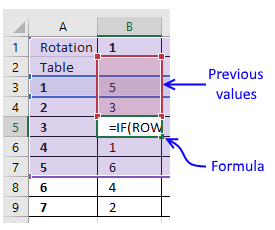
Array formula in cell B5:

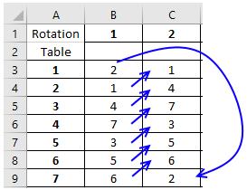
I tweaked the formula so it also considers previous values horizontally to make sure a table never has a duplicate group number, see picture below.

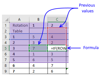
Here is the entire table, the formulas return almost always a #num error somewhere in the table. Press F9 to recalculate values if you have the attached workbook open.

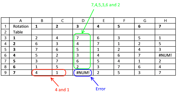
So why is this happening? Look at cell D9, number 4 and 1 is to the left of cell D9. This means that only numbers 2,3,5,6 or 7 can be populated in cell D9 or there will be a duplicate on row 9.

In this case, the values above cell D9 are 7,4,5,3,6 and 2 so the only value left is 1 or there will be a duplicate in column D. Number 1 is not possible in cell D9 so the formula returns a #NUM error.

The formulas above cell D9 do not take this into consideration while producing a random value, they only look back at previous values. It is not possible for the formulas to look at cells below or to the right because excel calculates each cell in this order.

It begins with the upper most left cell containing a formula, in this case B2 and then continues with the next cell below and so on, until there are no more formulas in that column. Excel then continues with the first formula in the next column, in this case cell C2.

Back to top

3. Formula - not random

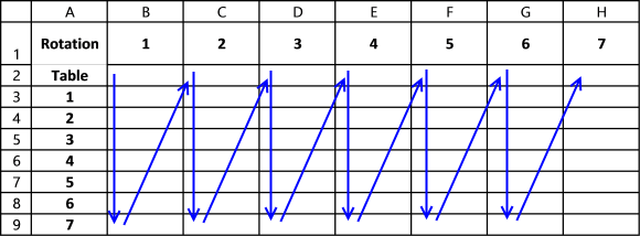
My second attempt to solve this problem is to move each value one cell for each rotation, the picture below shows how in the second rotation.

The problem with this approach is that only the first rotation has random values, the remaining rotations are not random. However, this technique makes it absolutely certain that a table has no repeats. Perhaps it is random enough?

Formula in cell C3:

To make it even more random I changed the formula so the first value in each column is random (row 3) but the sequence is the same as in rotation 1 (column B). As before, it takes previous values horizontally into account when calculating a new unique value.

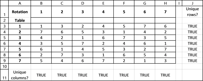
Array formula in cell B3:

Copy cell B3 and paste to cell range B4:B9.

Back to top

Explaining formula in cell B3

Step 1 - Create array containing a sequence from 1 to 7

The ROW function returns a number representing the row number of a cell reference.

ROW($1:$7)

returns {1; 2; 3; 4; 5; 6; 7}.

Step 2 - Count numbers in column B based on sequence 1 to 7

This step checks that previous cells above is not repeated again.

Cell reference $B$2:B2 grows when cell B3 is copied and pasted to cells below.

The COUNTIF function counts cells that are equal to a condition or criteria.

COUNTIF($B$2:B2, ROW($1:$7))

becomes

COUNTIF($B$2:B2, {1; 2; 3; 4; 5; 6; 7})

becomes

COUNTIF(0, {1; 2; 3; 4; 5; 6; 7})

and returns {0; 0; 0; 0; 0; 0; 0}.

Step 3 - Check if number in array is erqual to 0 (zero)

The equal sign compares the values in the array to 0 (zero), the result is either TRUE or FALSE.

COUNTIF($B$2:B2, ROW($1:$7))=0

becomes

{0; 0; 0; 0; 0; 0; 0}=0

and returns {TRUE; TRUE; TRUE; TRUE; TRUE; TRUE; TRUE}.

Step 4 - Convert boolean value to numerical value

The SUM function is not able to add boolean values, we need to convert the boolean values to their numerical equivalents. TRUE = 1 and FALSE = 0 (zero).

--(COUNTIF($B$2:B2, ROW($1:$7))=0)

becomes

--({TRUE; TRUE; TRUE; TRUE; TRUE; TRUE; TRUE})

and returns {1; 1; 1; 1; 1; 1; 1}.

Step 5 - Sum numerical values

The SUM function adds numerical values and ignores text and blanks, it then returns the total.

SUM(--(COUNTIF($B$2:B2, ROW($1:$7))=0))

becomes

SUM({1; 1; 1; 1; 1; 1; 1})

and returns 7.

Step 6 - Create a raandom number between 1 and the sum

The RANDBETWEEN function returns a number between a bottom number and a top number.

RANDBETWEEN(bottom, top)

RANDBETWEEN(1, SUM(--(COUNTIF($B$2:B2, ROW($1:$7))=0)))

becomes

RANDBETWEEN(1, 7)

and returns 7 (or any number between 1 and 7).

Step 7 - Extrakt the k-th largest number

The LARGE function returns the k-th largest number ina cell range or array.

LARGE(array, k)

LARGE((COUNTIF($B$2:B2, ROW($1:$7))=0)*ROW($1:$7), RANDBETWEEN(1, SUM(--(COUNTIF($B$2:B2, ROW($1:$7))=0))))

becomes

LARGE({1; 2; 3; 4; 5; 6; 7}, 7)

and returns 1.

Step 8 - Check if the current cell is less than eight

The ROW function returns a number representing the row number of a cell reference.

ROW(1:1)<8

becomes

1<8

The less than character checks if a number is lees than another number.

1<8

returns TRUE.

Step 9 - Return nothing if larger current cell is larger than seven

The IF function returns one value if the logical test is TRUE and another value if the logical test is FALSE.

IF(logical_test, [value_if_true], [value_if_false])

IF(ROW(1:1)<8, LARGE((COUNTIF($B$2:B2, ROW($1:$7))=0)*ROW($1:$7), RANDBETWEEN(1, SUM(--(COUNTIF($B$2:B2, ROW($1:$7))=0)))), "")

becomes

IF(ROW(1:1)<8, 1, "")

becomes

IF(TRUE, 1, "")

and returns 1.

Back to top

Array formula in cell C3:

Copy cell C3 and paste to cell range C3:H9.

Back to top

Get the Excel file

Rotating-unique-groups-with-no-repeatv2.xlsx

4. User defined function

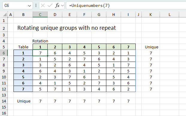
The User defined function in cell C6 returns an array of random unique numbers from 1 to n. The numbers are unique and random both vertically and horizontally. It allows you to specify the number rows and columns you want, however, it takes a lot of time trying to find random unique numbers that meet the conditions if you use a large value. A number greater than 7 may take a while to process.

The formulas in cells K6:K12 and B14:I14 calculates the number of random unique values for each row and column, to makes sure the UDF produces the desired array.

Function RndArray(n As Integer) As Variant
' Function to create and shuffle an array of numbers from 1 to n
    Dim arr() As Integer
    Dim i As Integer, j As Integer
    Dim tempValue As Integer

    ' Create the array with numbers from 1 to n
    ReDim arr(1 To n)
    For i = 1 To n
        arr(i) = i
    Next i

    For i = n To 2 Step -1
        j = WorksheetFunction.RandBetween(1, i)
        
        tempValue = arr(i)
        arr(i) = arr(j)
        arr(j) = tempValue
    Next i

    ' Return the shuffled array
    RndArray = arr
End Function

Function Uniquenumbers(m As Integer) As Variant
    Dim num As Variant
    Dim tempValue As Variant
    Dim i As Integer, j As Integer
    ReDim num(1 To m, 1 To m)
    tempValue = RndArray(m)
    
    'Save numbers to first column
    For i = 1 To m
        num(i, 1) = tempValue(i)
    Next i
    
    For i = 2 To m
start_new:
        tempValue = RndArray(m)
        For j = 1 To m
            For k = 1 To i - 1
                If num(j, k) = tempValue(j) Then
                    GoTo start_new
                Else
                    num(j, i) = tempValue(j)
                End If
            Next k
        Next j
    Next i

    Uniquenumbers = num
End Function

4.1 Where to copy the code?

You must copy the code to your workbook before you can run the code. Go to tab "Developer".

How to enable the "Developer" tab

Here is how to enable the "Developer" tab if it is missing.

1. Press with left mouse button on "File" located above the ribbon, a new pane appears.
2. Press with mouse on the "Options" button to access Excel settings.
3. Press with mouse on "Customize Ribbon" and then on the right side press with left mouse button on the checkbox next to the tab "Developer" to enable it.
4. Press with left mouse button on "OK" button to apply changes.

The "Developer" tab is now visible on the ribbon.

How to open Visual Basic Editor

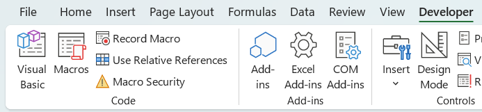
1. Go to tab "Developer" on the ribbon.
2. Press with left mouse button on the "Visual Basic" button to open the "Visual Basic Editor" (VBE). You can also press Alt + F11 to open VBE.

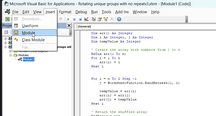
How to insert a module

1. Select the workbook in the "Explorer" window.
2. Press with left mouse button on "Insert" on the ribbon.
3. Press with left mouse button on "Module". A module appears below the workbook name in the "Explorer" window. See the image above.
4. Select the module.
5. Copy/Paste the VBA code above to the code window, see the image above.

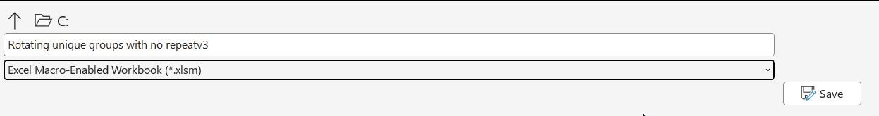
How to save the workbook as a macro-enabled workbook

1. Press with left mouse button on "File".
2. Press with left mouse button on "Save As...".
3. Type a file name.
4. Select file extension "Excel Macro-Enabled Workbook (*.xlsm).
5. Press with left mouse button on "Save" button.

This allows VBA code to be saved in the workbook.

How to enter the User Defined Function

Exit the Visual Basic Editor and go back to the worksheet. Type =Uniquenumbers(7) in a cell to populate the adjacent cells with a range containing 7 rows and 7 columns.

Final words

The UDF is actually brute-forcing different random arrays until one fits, this continues column by column. This makes it slow but it also leaves room for improvement.

Back to top

Permutations category

Find numbers closest to sum
Excelxor is such a great website for inspiration, I am really impressed by this post Which numbers add up to […]

How to create permutations
I discussed the difference between permutations and combinations in my last post, today I want to talk about two kinds […]

Excel categories

Comments (10)