Team Generator

Table of Contents
1. Team Generator
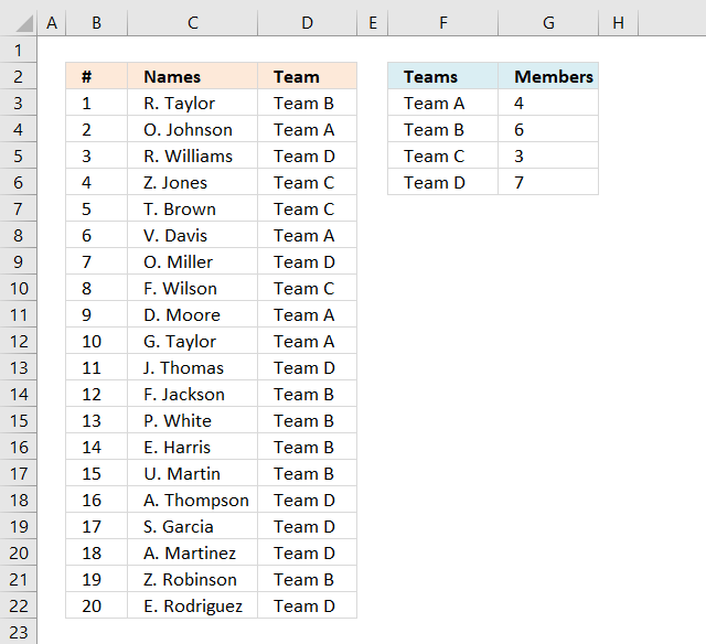
This section describes how to create teams randomly. There are twenty names in column B and four teams in column E. There will be five team members in each team. In column C a team is randomly selected in each cell.
Excel 365 dynamic array formula in cell C2:
The formula above references values in cell E2:E5 which I first converted to an Excel defined table named Table1. This makes the formula dynamic meaning it recalculates automatically based on the number of entries in Table1.
The formula above spills values to cells below C2 as far as needed, a #SPILL error indicates that the cells below C2 are not empty. Delete nonempty cells and the formula works again.
Array formula in cell C2 for earlier Excel versions:
How to create an array formula
- Copy the aray formula above (Ctrl + c)
- Double press with left mouse button on cell B2
- Paste (Ctrl + v)
- Press and hold Ctrl + Shift simultaneously
- Press Enter
- Release all keys
If you made the above steps correctly the formula now has a beginning and ending curly bracket, like this:
{=array_formula}
Don't enter these characters yourself, they appear automatically.
Customize formula
COUNTIF($C$1:C1, $E$2:$E$5)<5 makes sure that each team has max five team members.
ROW($1:$4) gives a row number to each team. Example, if you have three teams, change it to ROW($1:$3) or the formula won't work.
Explaining formula in cell C2
Step 1 - Make sure that not more than 5 names have been assigned the same team
The COUNTIF function counts values based on a condition or criteria, the first argument contains an expanding cell reference, it grows when the cell is copied to cells below. This makes the formula aware of values displayed in cells above.
COUNTIF($C$1:C1, $E$2:$E$5)<5
becomes {0; 0; 0; 0}<5
and returns {TRUE; TRUE; TRUE; TRUE}.
Step 2 - Multiply with array containing row numbers
(COUNTIF($C$1:C1, $E$2:$E$5)<5)*(ROW($1:$4))
becomes {TRUE; TRUE; TRUE; TRUE}*{1;2;3;4}
and returns {1;2;3;4}
Step 3 - Extract random row number
The LARGE function returns the k-th largest number, k is calculated based on how many teams that have been shown up until this cell.
LARGE((COUNTIF($C$1:C1, $E$2:$E$5)<5)*(ROW($1:$4)), RANDBETWEEN(1, SUMPRODUCT(--(COUNTIF($C$1:C1, $E$2:$E$5)<5))))
SUMPRODUCT function returns the number of team names that have not yet been fully assigned to players.
LARGE({1;2;3;4}, RANDBETWEEN(1, SUMPRODUCT(--({TRUE; TRUE; TRUE; TRUE}))))
becomes LARGE({1;2;3;4}, 3)
and returns 3. This is a random number.
Step 4 - Return value
The INDEX function returns a value based on a cell reference and column/row numbers.
INDEX($E$2:$E$5, LARGE((COUNTIF($C$1:C1, $E$2:$E$5)<5)*(ROW($1:$4)), RANDBETWEEN(1, SUMPRODUCT(--(COUNTIF($C$1:C1, $E$2:$E$5)<5)))))
returns "Team C" in cell C2.
This article demonstrates how to generate teams of different sizes:
Recommended articles
JD asks in this post: Dynamic team generator Hi, what if we have different number of people per team? So in […]
The following shows you how to set up a dynamic scoreboard, enter results and the scoreboard is automatically recalculated:
Recommended articles
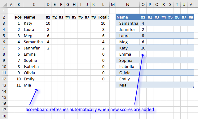
This article demonstrates a scoreboard, displayed to the left, that sorts contestants based on total scores and refreshes instantly each […]
2. Dynamic team generator
Mark G asks:
1 - I see you could change the formula to have the experssion COUNTIF($C$1:C1, $E$2:$E$5)<5 changed so the maximum number of team members looks to a cell (say E9) so the number of people per team could be easily changed eg COUNTIF($C$1:C1, $E$2:$E$5)<E9
2 - In (virtual) sailing team racing, competition is usually 3 vs 3, but could be adjusted to a 4 vs 4, 3 vs 2 or 4 vs 3 depending on the number of skippers available to race. Could the example be modified to assign a skipper to a team given these optimum arrangements? (eg for say 12 skippers entered it would do 2 sets of 3 vs 3, for 8 skippers it would do one 4 vs 4, etc)
Answer:
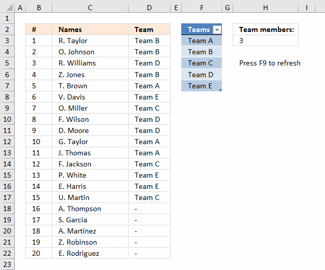
The image above demonstrates a worksheet containing Team names in an Excel defined table cell range F3:F7, you don't need to adjust cell references in the formula if you add or delete team names. It is dynamic and updates instantly.
Enter the number of members in each team in cell H3, the formula refreshes automatically. It randomly assigns teams to players, press F9 to refresh the formula output.
Array formula in cell D3:
To enter an array formula, type the formula in a cell then press and hold CTRL + SHIFT simultaneously, now press Enter once. Release all keys.
The formula bar now shows the formula with a beginning and ending curly bracket telling you that you entered the formula successfully. Don't enter the curly brackets yourself.
Copy cell D3 and paste it down as far as necessary.
Explaining formula in cell D3
Step 1 - Count previous values
The COUNTIF function counts values based on a condition or criteria, the first argument contains an expanding cell reference, it grows when the cell is copied to cells below. This makes the formula aware of values displayed in cells above. 0 (zero) indicates values that not yet have been displayed.
COUNTIF($D$2:D2, Table1[Teams])<$H$3
becomes
COUNTIF("Team", {"Team A"; "Team B"; "Team C"; "Team D"; "Team E"})<$H$3
becomes
{0;0;0;0;0}<3
and returns
{TRUE; TRUE; TRUE; TRUE; TRUE}
Step 2 - Create row numbers
This step is needed to create a sequence of numbers that will be used to get the correct value in a later step.
MATCH(ROW(Table1[Teams]),ROW(Table1[Teams]))
returns {1;2;... ;5}.
Step 3 - Multiply arrays
(COUNTIF($D$2:D2, Table1[Teams])<$H$3)*(MATCH(ROW(Table1[Teams]),ROW(Table1[Teams])))
returns {1;2;3;4;5}.
Step 4 - Extract random row number
The LARGE function returns the k-th largest number, LARGE( array , k). The second argument k is a random number from 1 to n.
LARGE((COUNTIF($D$2:D2, Table1[Teams])<$H$3)*(MATCH(ROW(Table1[Teams]),ROW(Table1[Teams]))), RANDBETWEEN(1, SUMPRODUCT(--(COUNTIF($D$2:D2, Table1[Teams])<$H$3))))
becomes LARGE({1;2;3;4;5}, 2) and returns 2. This is a random number between 1 and 5.
Step 5 - Return value
The INDEX function returns a value based on a cell reference and column/row numbers.
INDEX(Table1[Teams], LARGE((COUNTIF($D$2:D2, Table1[Teams])<$H$3)*(MATCH(ROW(Table1[Teams]),ROW(Table1[Teams]))), RANDBETWEEN(1, SUMPRODUCT(--(COUNTIF($D$2:D2, Table1[Teams])<$H$3)))))
becomes
INDEX(Table1[Teams], 2)
and returns "Team B" in cell D3.
Step 6 - Trap errors
The formula returns errors when all teams are populated, the IFERROR function converts the errors into a given value, in this case "-".
IFERROR(INDEX(Table1[Teams], LARGE((COUNTIF($D$2:D2, Table1[Teams])<$H$3)*(MATCH(ROW(Table1[Teams]),ROW(Table1[Teams]))), RANDBETWEEN(1, SUMPRODUCT(--(COUNTIF($D$2:D2, Table1[Teams])<$H$3))))), "-")
3. How to build a Team Generator - different number of people per team
Hi, what if we have different number of people per team? So in team A, there could be a max of 4 members but in team B there could be a max of 6 members etc. Is there some formula which can be used for this as well?
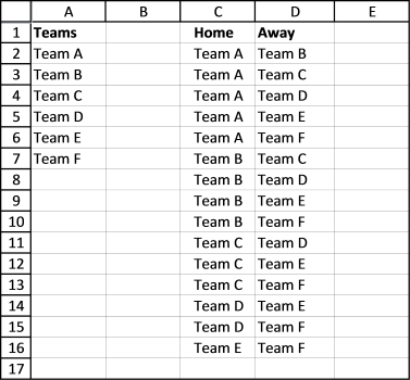
Yes, there is. This array formula uses the values in cell range D2:E4 to randomly assign people to teams, demonstrated in column B and C.
<>3.1. Team Generator - formula
The image above shows a formula in column D that assigns teams to names randomly based on the number of team members specified in column G.
Change the team names in column F if you like and type a number in the corresponding cell in column G to force the formula to assign a maximum number of team members.
Array formula in cell D3:
This array formula contains a couple of excel functions, if you want to know more about them check out these posts: LARGE, INDEX, COUNTIF, IFERROR, MATCH, ROW, RANDBETWEEN. It also has both absolute and relative cell references, learn more.
3.1.1 How to enter an array formula
- Copy above array formula
- Select cell C2
- Paste array formula to the formula bar
- Press and hold CTRL + SHIFT simultaneously
- Press Enter once
If you did it right the formula now begins and ends with curly brackets, like this {=array formula}. Don't enter the curly brackets yourself.
3.1.2 How to copy the formula to cells below
- Select cell C2
- Copy cell (Shortcut key CTRL + c)
- Select cell range C3:C21
- Paste (Shortcut key CTRL + v)
You can also select cell C2, press and hold on the black dot on the lower right corner of cell C2. Drag it down as far as needed.
3.1.3 Named ranges in the array formula

There are two named ranges in this worksheet, Teams and Members. They return a cell range in column F and G respectively that grow automatically as you add new values.
3.1.4 How to create a named range
- Copy formula below.
- Go to tab Formula on the ribbon.
- Press with left mouse button on the "Name Manager" button. A dialog box appears.
- Press with left mouse button on the "New..." button located on the dialog box. Another dialog box appears.
- Paste formula to "Refers to;" field.
- Name the named range in "Name:" field.
- Press with left mouse button on OK button.
- Repeat steps 4 to 7 to create the second named range.
- Press with left mouse button on OK button on the first dialog box to apply changes and dismiss it.
Teams:
Members:
3.1.5 Explaining formula in cell D3
IFERROR(INDEX(Teams, LARGE((COUNTIF($D$2:D2, Teams)<>Members)*MATCH(ROW(Teams), ROW(Teams)), RANDBETWEEN(1, SUM(--(COUNTIF($D$2:D2, Teams)<>Members))))), "")
Step 1 - Count previous teams in cells above
The COUNTIF function calculates the number of cells that are equal to a condition.
COUNTIF(range, criteria)
The first argument is a cell reference that contains both a relative and absolute part meaning the cell ref grows when cell is copied to cells below.
The second argument is a dynamic named range meaning it grows when more values are added.
COUNTIF($D$2:D2, Teams)
becomes
COUNTIF("Team", {"Team A"; "Team B"; "Team C"; "Team D"})
and returns {0; 0; 0; 0}.
Step 2 - Check if value is not equal to the total number of members in a team
The less than and larger than character combined means not equal to. This step makes sure that there is a correct number of assigned team members.
COUNTIF($D$2:D2, Teams)<>Members
becomes
{0;0;0;0}<>Members
becomes
{0;0;0;0}<>{4;6;3;7}
and returns {TRUE; TRUE; TRUE; TRUE}
Step 3 - Convert boolean values to numerical
This step converts TRUE to 1 and FALSE to 0 (zero).
--(COUNTIF($D$2:D2, Teams)<>Members)
becomes
--({TRUE; TRUE; TRUE; TRUE})
and returns {1; 1; 1; 1}. This step is needed to be able to calculate a sum.
Step 4 - Calculate total
The SUM function adds numbers from a cell range or an array and returns a total. It can't, however, sum boolean values.
SUM(--(COUNTIF($D$2:D2, Teams)<>Members))
becomes
SUM({1; 1; 1; 1})
and returns 4.
Step 5 - Create a random number based on Team member count
The RANDBETWEEN function returns a random whole number between the numbers you specify.
RANDBETWEEN(bottom, top)
RANDBETWEEN(1, SUM(--(COUNTIF($D$2:D2, Teams)<>Members))))
becomes
RANDBETWEEN(1, 4)
and returns a pseudo-random number from 1 to 4.
Step 6 - Create an array from 1 to n
The ROW function returns the row number from a cell reference, if a cell range is used all numbers are returned in an array.
MATCH(ROW(Teams), ROW(Teams))
becomes
MATCH({3;4;5;6}, {3;4;5;6})
The MATCH function finds the relative position of a given value in a cell range or array. This step makes sure the array begins with 1.
MATCH({3;4;5;6}, {3;4;5;6})
returns {1;2;3;4}.
Step 7 - Extract k-th largest value
The LARGE function extracts the k-th largest number from an array or cell range.
LARGE(array, k)
LARGE((COUNTIF($D$2:D2, Teams)<>Members)*MATCH(ROW(Teams), ROW(Teams)), RANDBETWEEN(1, SUM(--(COUNTIF($D$2:D2, Teams)<>Members))))
becomes
LARGE((COUNTIF($D$2:D2, Teams)<>Members)*MATCH(ROW(Teams), ROW(Teams)), 3)
becomes
LARGE(({TRUE; TRUE; TRUE; TRUE})*MATCH(ROW(Teams), ROW(Teams)), 3)
becomes
LARGE(({TRUE; TRUE; TRUE; TRUE})*{1;2;3;4}, 3)
becomes
LARGE(({TRUE; TRUE; TRUE; TRUE})*{1;2;3;4}, 3)
becomes
LARGE({1;2;3;4}, 3)
and returns 2.
Step 8 - Get value
The INDEX function returns a value from a cell range based on a row and column number (optional).
INDEX(Teams, LARGE((COUNTIF($D$2:D2, Teams)<>Members)*MATCH(ROW(Teams), ROW(Teams)), RANDBETWEEN(1, SUM(--(COUNTIF($D$2:D2, Teams)<>Members)))))
becomes
INDEX(Teams, 2)
becomes
INDEX({"Team A";"Team B";"Team C";"Team D"}, 2)
and returns "Team B" in cell D3.
Step 9 - Check if value is an error
The IFERROR function handles errors, you can specify what value to returns if an error is found.
IFERROR(value, value_if_error)
IFERROR(INDEX($F$3:$F$19, LARGE((COUNTIF($D$2:D2, Teams)<>Members)*MATCH(ROW(Teams), ROW(Teams)), RANDBETWEEN(1, SUM(--(COUNTIF($D$2:D2, Teams)<>Members))))), "")
becomes
IFERROR("Team B", "")
and returns "Team B".
1.6 Disable automatic recalculation
The RANDBETWEEN function is volatile and each time you enter a new value somewhere on this sheet, array formulas are recalculated.
To prevent this from happening the following event code turns off automatic calculation. Activating sheet1 enables manual calculation, deactivating sheet1 enables automatic calculation.
Private Sub Worksheet_Activate()
Application.Calculation = xlCalculationManual
End Sub
Private Sub Worksheet_Deactivate()
Application.Calculation = xlCalculationAutomatic
End Sub
Where is this code? Press with right mouse button on on tab sheet1. Press with mouse on "View Code..."
Remember to press F9 after editing teams and member columns.
Want to learn more about advanced excel techniques, join my Advanced excel course.
These posts use the same technique:
Random category
This article demonstrates macros that create different types of round-robin tournaments. Table of contents Basic schedule - each team plays […]
Team generator category
More than 1300 Excel formulasExcel categories
25 Responses to “Team Generator”
Leave a Reply
How to comment
How to add a formula to your comment
<code>Insert your formula here.</code>
Convert less than and larger than signs
Use html character entities instead of less than and larger than signs.
< becomes < and > becomes >
How to add VBA code to your comment
[vb 1="vbnet" language=","]
Put your VBA code here.
[/vb]
How to add a picture to your comment:
Upload picture to postimage.org or imgur
Paste image link to your comment.
1 - I see you could change the formula to have the experssion COUNTIF($C$1:C1, $E$2:$E$5)<5 changed so the maximum number of team members looks to a cell (say E9) so the number of people per team could be easily changed eg COUNTIF($C$1:C1, $E$2:$E$5)<E9
2 - In (virtual) sailing team racing, competition is usually 3 vs 3, but could be adjusted to a 4 vs 4, 3 vs 2 or 4 vs 3 depending on the number of skippers available to race. Could the example be modified to assign a skipper to a team given these optimum arrangements? (eg for say 12 skippers entered it would do 2 sets of 3 vs 3, for 8 skippers it would do one 4 vs 4, etc)
Mark G,
read this post: Dynamic team generator in excel
The is a fabulous tool! I used it for generating business simulation teams for a leadership development exercise at work. It worked great! Thank you so much!
Lisa Liszcz,
Thank you, I am happy you like it!
Great post, worked really well. Used it in business competition teams assignments. Appreciate sharing the knowledge, thanks so much !
Hi, what if we have different number of people per team? So in team A, there could be a max of 4 members but in team B there could be a max of 6 members etc. Is there some formula which can be used for this as well?
JD
Read this post: https://www.get-digital-help.com/team-generator/
In a scenario like this and recalculating the setup several times, I see that the Team A is never assigned to #10 or greater. Is this a limitation?
Felipe Costa Gualberto,
This workbook assigns teams evenly.
https://www.get-digital-help.com/wp-content/uploads/2015/04/Team-Generatorv2.xlsm
I'm trying to upload the image, but I can't.
The link would be: https://s24.postimg.org/iy5s86r8l/Sem_t_tulo.png
However, the setup I did was just 1 member in Team A and 19 members in Team B.
Felipe Costa Gualberto,
If there are two teams, the probability is 50% that a team is displayed in a cell, that is why Team B is shown almost always in one of the three or four first cells. This is perhaps not ideal, I am working on a better formula.
I have a question that may be more complex, but similar in theory.
This is for a team building exercise in my classroom.
I have 18 students. I want to generate groups of 3 that will allow each person to work with 2 unique people each time, with no repeats. I think this would mean 8 groups of 3, and 1 group of 2. Or, 7 groups of 3, and 1 group of 4.
Does this make sense? Can anyone help?
What if one of those names were to be absent, how would you write the code if say cell B4 was left blank an the generator didn't count them on a team?
Great tool! I'm trying to understand how the formula works. Could someone explain what this part of the formula does?
COUNTIF($C$1:C1, OFFSET($D$2:$D$5, 0, 0, $F$1))<$F$2
I understand what the COUNTIF and OFFSET commands do, but I don't get how they are being used in this part of the formula
I play a vball league where We'd like to have a spreadsheet that we plug the 16 names (8 guys + 8 girls) into, and it produces randomly generated teams based on the following:
1. We play 8 games
1. 2 guys and 2 girls per team
2. Cannot be paired with any another player more than 3 times.
3. It would be nice to be paired with all other players at least once during the 8 games.
Hi Oscar,
Do you have a template for 60 people to be randomly generated into teams of 4?
Thanks,
Vlad
[…] }); Check the below links.. Hope it might give you a solution. Team Generator in excel | Get Digital Help - Microsoft Excel resource […]
How would you change the name list to be dynamic such as 20 one time then 43 another and so on and then make teams of 4 with odd leftovers in a team ? Of course, no limit on number of teams just whatever it takes.
Hello,
I am trying to adjust the formula to have people for 6 teams. There are actually three teams of 2, but I want to assign specific positions for each team, so I am making it 6 teams in excel. For example, Team one would have a forward and a goalie, so in excel I am making it 2 teams, G1 and F1. I want to have 6 people, 6 teams, so everyone is assigned a position and team. I keep trying to edit the formula to let me do this but I keep getting #NUM! in the team assignment sections. What could I be doing wrong?
I change the COUNTIF($C$1:C1, $E$2:$E$5)<5 to <1
And I change the ROW($1:$4) to ROW($1:$6)
Any suggestions?
Thanks
Hi,
I plan to use something like this so people can sign up for football on a Google sheet. Is it possible to get a team member assigned a team at random as they sign up?
So 2 teams of 7, assigned Team A or B as they sign up, and also prevent it from recalculating on change.
Cheers!
Oliver
Hi Oliver
Is it possible to get a team member assigned a team at random as they sign up? So 2 teams of 7, assigned Team A or B as they sign up, and also prevent it from recalculating on change.
I believe you need a macro to do that.
Hi Oscar, how would you do this with an additional level of criteria? For example, if your participants are also in categories: A, B & C and in Group 1 you want 3 Category A participants, 2 Category B, etc.
Hi,
How to do this without being random?
What I mean is, I am looking to divide a bunch of soccer players in 3 teams. Each player has a rating, position he pays for and availability as parameters.
Now how can I distribute them evenly in each team so that all the skill-sets and ratings of all the available players are distributed evenly?
The flow for it is as follows:
1) First it needs to check availability
2) Sort the all the Goalkeepers in 3 teams
3) Then all strikers and then all defenders to be distributed
Every week for a season, the only input that will change will be availability rest everything will be same.
Sorry for asking such a lengthy question, but have been trying to solve it form a really long time.
I really appreciate your effort. I have been trying to build a team generator for my class room assignment work, so that students can't pick only those friends who they are attached with. Otherwsie, they are not gonna learn the team building. This Post has made the work much easier for myself.