Plot date ranges in a calendar
Table of Contents
1. Plot date ranges in a calendar
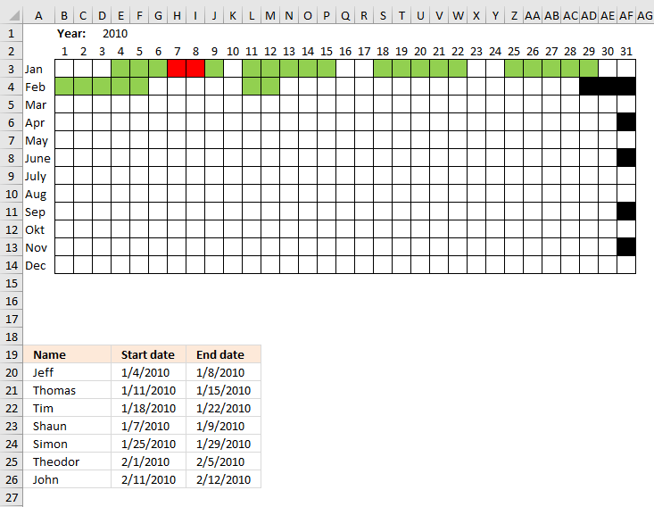
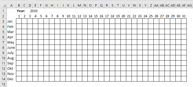
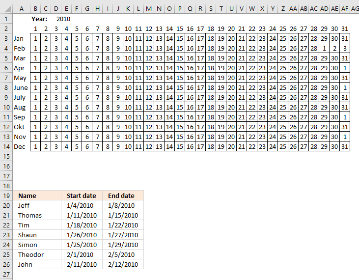
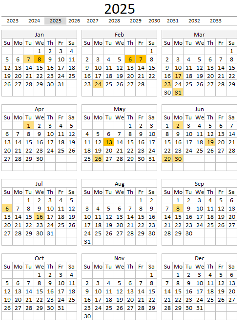
The image above demonstrates cells highlighted using a conditional formatting formula based on a table containing date ranges.
The calendar lets you choose year in cell D1 and the highlighted cells changes accordingly and immediately. The months are in column A and days of the days of the months are in row 2.
Check out this article Heat map yearly calendar if you want to highlight date ranges in yearly view.
This post Yet another excel calendar has a different layout yet still showing all dates in a year. There is also a monthly and daily view, however it won't allow you to add date ranges only single day events.
The following calendar Calendar – monthly view plots the events in a day instead of highlighting days.
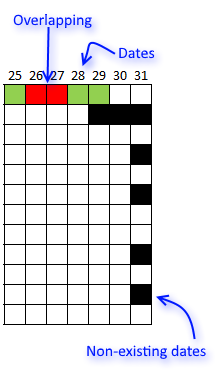 I have used Conditional Formatting to
- highlight date ranges (green)
- highlight overlapping dates (red)
- not existing dates (black)
demonstrated in the image to the right.
The conditional formatting formula updates as you type new date ranges or edit an existing one in the table.
This gives you an overview of the date ranges that lets you easily spot any issues or errors.
How I created "invisible" dates in cell range B3:AF14
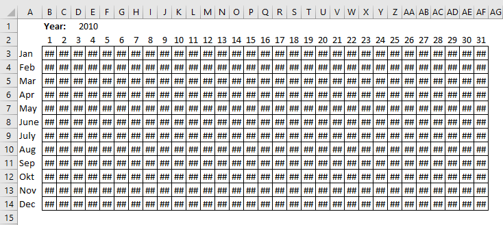
- Formula in B3: =DATE($D$1;ROWS($A$3:$A3);B$2) + ENTER.
$D$1 is an absolute reference to a cell containing a year. - Copy cell B3 and paste into cell range B3:AF14.

Excel tries to output the entire date but the cell width is too small. That is why it looks like it does, in the image above. - Select B3:AF14
- Press CTRL + 1
- Select "Number" tab
- Select "Custom"
- Type ,,, in "Type:" window
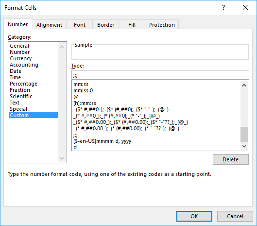
- Press with left mouse button on OK!
The steps above hide the dates in cell range B3:AF14.
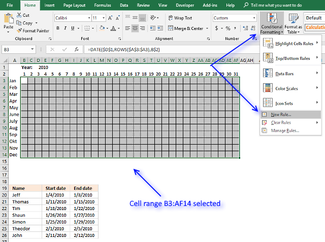
How to highlight date ranges green
- Select B3:AF14.
- Press with left mouse button on "Home" tab
- Press with left mouse button on "Conditional formatting" button
- Press with left mouse button on "New Rule.."
- Select "Use a formula to determine which cells to format"
- Type in "Format values where this formula is true" window: =SUMPRODUCT((B3<=$I$19:$I$26)*(B3>=$E$19:$E$26))=1
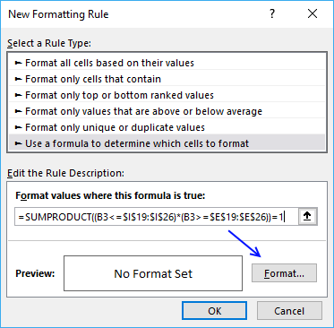
- Press with left mouse button on "Format.." button
- Press with left mouse button on "Fill" tab
- Select a color (green)
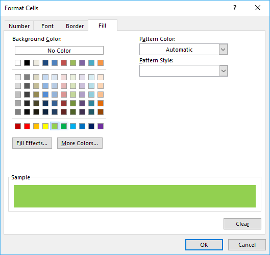
- Press with left mouse button on OK!
- Press with left mouse button on OK!
- Press with left mouse button on OK!
The CF formula in step 6 above checks if the date is inside any of the date ranges, if exactly one date range is then the date cell is highlighted green.
How to highlight overlapping date ranges red
The steps here are identical to the steps above, however, the CF formula is different.
- Select B3:AF14.
- Press with left mouse button on "Home" tab
- Press with left mouse button on "Conditional formatting" button
- Press with left mouse button on "New Rule.."
- Select "Use a formula to determine which cells to format"
- Type in "Format values where this formula is true" window: =SUMPRODUCT((B3<=$I$19:$I$26)*(B3>=$E$19:$E$26))>1
- Press with left mouse button on "Format.." button
- Press with left mouse button on "Fill" tab
- Select a color (red)
- Press with left mouse button on OK!
- Press with left mouse button on OK!
- Press with left mouse button on OK!
The CF formula in step 6 above checks if the date is inside any of the date ranges, if more than one date ranges are then the date cell is highlighted red.
How to highlight not existing dates black
- Select B3:AF14.
- Press with left mouse button on "Home" tab
- Press with left mouse button on "Conditional formatting" button
- Press with left mouse button on "New Rule.."
- Select "Use a formula to determine which cells to format"
- Type in "Format values where this formula is true" window:=MONTH(B3)<>ROWS($B$3:$B3)
- Press with left mouse button on "Format.." button
- Press with left mouse button on "Fill" tab
- Select a color (black)
- Press with left mouse button on OK!
- Press with left mouse button on OK!
- Press with left mouse button on OK!
The formula in step 6 above checks that the month number is equal to the row number returned by the ROWS function. This makes sure that the date is in the correct month and not in the next month.
If it is in the next month then the cell is colored black. The following image shows the days of the months. For example, February 2010 has 28 days, the formula starts with 1 March in the next cell to the right of 28.
To hide that the cell is colored black.
How to reorder conditional formatting rules
- Press with left mouse button on "Home" tab
- Press with left mouse button on "Conditional formatting" button
- Press with left mouse button on "Manage Rules.."
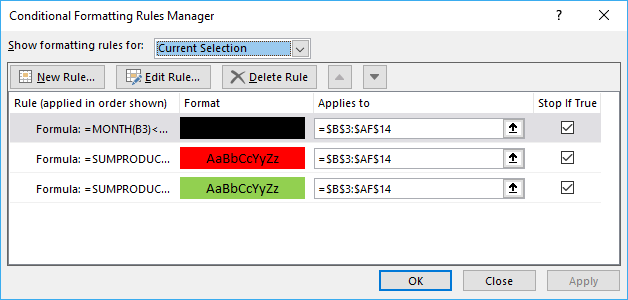
- Reorder rules using arrow buttons
Rule (applied in the order shown)
- Black
- Red
- Green
Conditional Formatting formulas
You will find an explanation in greater detail here:
Highlight overlapping date ranges using conditional formatting
2. Plot date ranges in a calendar part 2
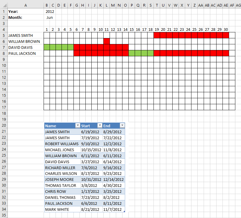
I will in this section demonstrate a calendar that automatically highlights dates based on date ranges, the calendar populates names and corresponding dates based on the month and year selected by the user.
This is a new version of Visualize date ranges in a calendar. The workbook in this section lets you enter names and date ranges in an Excel defined Table. It allows you to add or delete names and date ranges without changing the cell references in the formulas.
Duplicate names are allowed, select year and month, days in that month are automatically calculated (row 4) and displayed accordingly.
Names whose date ranges are present in the selected month are displayed in cell range A5:A17. Dates are red if they overlap with another date range. This workbook contains no VBA code.
What you will learn in this section
- Create a dynamic monthly calendar.
- Create a calendar that highlights date ranges green and overlapping date ranges red.
- List names accordingly based on the corresponding date ranges.
- Build Conditional formatting formulas that highlight cells based on name and date.
- Build a formula that extracts names based on a year and month.
How this worksheet works
The animated image above shows when I select a month and the calendar instantly displays the appropriate names and dates based on the date ranges below the calendar.
Enter a value in cell B1 to change year, use the drop down list in cell B2 to select the month.
How I created this worksheet
Data list validation in cell B2
- Select cell B2
- Go to tab "Data"
- Press with left mouse button on "Data Validation" button

- Select List
- Type: Jan,Feb,Mar,Apr,May,Jun,Jul,Aug,Sep,Oct,Nov,Dec in Source:
- Press with left mouse button on OK button
Calculate first date in selected month in cell D1
Formula:
Calculate last date in selected month in cell D2
Formula:
Hide cell values in cell range D1:D2
These steps shows you how to hide values in a cell by applying cell formatting, the value is still there but you can't see it.
- Select cell range D1:D2
- Press Ctrl + 1
- Go to "Number" tab
- Press with left mouse button on "Custom"
- Type ;;;
- Press OK
Calculate dates
Formula in cell B4:
Formula in cell C4:
Copy cell C4 and paste to cell range D4:AF4.
Create an Excel defined Table
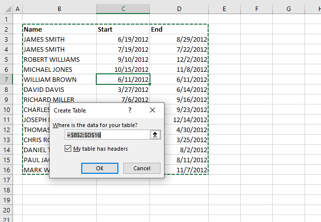
- Select any cell in the data set that contains names and date ranges.
- Press CTRL + T to open the "Create Table" dialog box.
- Press with left mouse button on OK button.
Filter names in column A
Array formula in cell A5:
- Copy above array formula
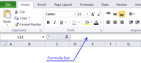
- Paste in formula bar
- Press and hold Ctrl + Shift
- Press Enter
- Copy cell A5 and paste to cell range A6:A17
Explaining array formula in cell A5
Step 1 - Identify records that overlap selected month
The less than and greater than signs are logical oerpators that allows you to compare the date ranges saved in the Excel defined Table to the hidden dates in cell D1 and D2.
Cell D1 contains the first date in the selected month and cell D2 contains the last date of the selected dates.
(Table1[Start]<=$D$2)*(Table1[End]>=$D$1)
returns {1;0;0;0;1;1;0;0;0;0;0;0;1;0}
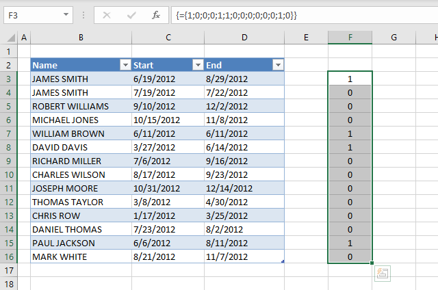
The position of each value matches the records in the Excel defined Table, for example, 1 indicates that the first record overlaps the select month June and year 2012.
0 (zero) tells us that the record does not overlap the selected year and month.
Step 2 - Convert boolean values to corresponding relative row number
The IF function lets you use a logical expression to determine which argument to return: value_if_true or value_if_false.
IF(logical_test, [value_if_true], [value_if_false])
IF((Table1[Start]<=$D$2)*(Table1[End]>=$D$1), MATCH(Table1[Start], Table1[Start], 0), "")
To create an array of numbers starting from 1 to the number of records in the Excel defined Table I use the MATCH and ROW functions.
The ROW function returns an array of numbers representing the row number for each record, however they don't start with 1 in most cases.
The MATCH function lets you convert the array to a sequence of numbers that start with 1.
returns
{1;"";"";"";5;6;"";"";"";"";"";"";13;""}.
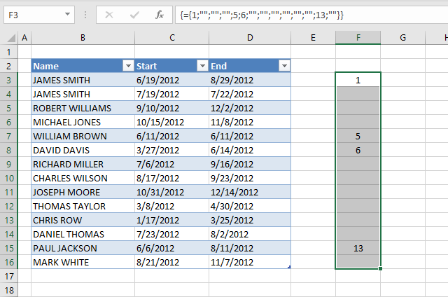
The image above shows the array next to the Excel defined Table. The array contains the relative row number of each record that overlaps the selected year and month.
Step 3 - Extract k-th smallest row number
In order to extract a new value in each cell I use the SMALL function with a relative cell reference that changes automatically when I copy the cell to cells below.
SMALL(array, k)
SMALL(IF((Table1[Start]<=$D$2)*(Table1[End]>=$D$1), MATCH(Table1[Start], Table1[Start], 0), ""), ROW(A1))
becomes
SMALL({1;"";"";"";5;6;"";"";"";"";"";"";13;""}, 1)
and returns 1.
Step 4 - Return name
The INDEX function returns a value from a given cell range based on a row and column number.
INDEX(Table1[Name], SMALL(IF((Table1[Start]<=$D$2)*(Table1[End]>=$D$1), MATCH(Table1[Start], Table1[Start], 0), ""), ROW(A1)))
becomes
INDEX(Table1[Name], 1)
and returns the first value in column Name which is James Smith.
Step 5 - Remove errors
When values run out the formula returns an error, the IFERROR function removes the errors and returns a blank cell instead.
For example, in cell A9 the formula becomes:
IFERROR(INDEX(Table1[Name], SMALL(IF((Table1[Start]<=$D$2)*(Table1[End]>=$D$1), MATCH(Table1[Start], Table1[Start], 0), ""), ROW(A5))), "")
becomes
IFERROR(#NUM!, "")
and returns a blank.
Red conditional formatting formula
Conditional formatting formula applied to cell range B5:AF17:
Green conditional formatting
Conditional formatting formula applied to cell range B5:AF17:
Recommended posts:
Visualize date ranges in a calendar in excel
Advanced Gantt Chart Template
3. Highlight events in a yearly calendar

This article demonstrates how to highlight given date ranges in a yearly calendar, this calendar allows you to change the year and the calendar dates change accordingly.
The image above shows an Excel Table to the right of the calendar, you can easily add as many events as you like.
This worksheet uses Conditional Formatting formulas containing structured references pointing to the Excel defined Table, this makes it simple to use because no formulas need to be changed when the list of events grows larger.
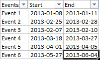
I got 6 events with different dates.
Event - DATE START - DATE END
1
2
3
4
5
6
On sheet 2 I have a Year Calander (365 Days). I need to do apply conditional formatting to highlight the days in which I have events.The six events are just a start and the list will grow longer. I want to have a pictorial view of the calendar on where the events fall in the year which is Sheet2.Sheet1 is just the key in the dates for the start and end.
How to create an Excel Table

The main benefit of converting the data set, in this case, is that the cell references in formulas don't need to be changed when you add additional date ranges to the Excel Table.
The cell references pointing to an Excel Table are called structured references and are dynamic, they don't change no matter how many date ranges you add to the Table.
One disadvantage with structured cell references is that you need to apply a workaround in order to use them in Conditional formatting formulas and Drop Down Lists.
- Select any cell in your data set.
- Press shortcut keys CTRL + T to open the "Create Table" dialog box, see image above.
- Press OK button to create the Excel Table.
How to build a dynamic yearly calendar based on input year

Here are the steps to create the calendar without dates.
- Select cell range B4:H4.
- Go to tab "Home" on the ribbon if you are not already there.
- Press with left mouse button on "Merge and Center" button.
- Type this formula in cell B4: =DATE($K$2,1,1) and press Enter. This will return a date, however, we need only the month name to be displayed.
- Select cell B4 and press CTRL + 1 to open the "Format Cells" dialog box.
- Select category: Custom and type mmmm.
- Press with left mouse button on OK button. This will format the date in cell B4 to only show the month name. This will make the month name dynamic meaning it will change if the Excel user has a different Excel language installed.
- Select cell B5 and type Mo and then press Tab key to move to the next cell.
- Continue typing Tu, We, Th, Fr, Sa and Su with the remaining cells, see image above.
- Press and hold on column header B.
- Drag with mouse to column H.
- Press and hold on any of the separating lines between the column headers.
- Drag with mouse until column width is around 26 pixels, you can change this later.
- Release mouse button and all selected columns will have the width 26 pixels.

- Copy cell range B4:H5 and paste to J4:P5.
- Change columns widths to 26 pixels.
- Enter this formula in cell J4 for February: =DATE($K$2,2,1)
The only difference between this formula and the formula for January is the month argument which I have bolded in the formula above.
2 represents February which is the second month.

- Copy cell range B4:X5 and paste to B13:X20.
- Change these months as well. March formula: =DATE($K$2,3,1)
- Repeat with remaining quarters.

The week starts with Sunday if you live in the US, the image then looks like this.

Select month names, weekday names and six rows below each month and apply a border to the selected cells.
- Go to tab "Home" on the ribbon.
- Press with mouse on border button.
- Press with mouse on "All borders".

This creates a border around each cell.

- Select columns B to X.
- Go to tab "Home" on the ribbon.
- Press with mouse on "Center" button to center cell content.

Calendar date formulas

I center and merged cell range K2:O2 and entered year 2020 as an example, all formulas will be based on this year that is entered in cell K2.
Select cell B6 which is the first cell for the month of January, type the following formula:
This formula calculates the first date in the first week which the first day in January falls, this may be a date in December, however, I will use Conditional formatting to hide dates outside the month later in this article.
The DATE function uses three arguments, year, month and day. DATE(year, month, day)
DATE($K$2,1,1)
becomes
DATE(2020,1,1)
and returns 12/30/2019.
The WEEKDAY function calculates a number based on a date representing the position in a week. WEEKDAY(serial_number,[return_type])
The serial_number argument is the date and the [return_type] argument lets you pick which day the week begins with. return_type 2 returns 1 for Monday, 2 for Tuesday, 3 for Wednesday, etc.
DATE($K$2,1,1)-WEEKDAY(DATE($K$2,1,1),2)+1
becomes
43831-WEEKDAY(43831,2)+1
1/1/2020 falls on a Wednesday and the WEEKNUM function will then return 3. 3 = Wednesday.
43831-3
and returns
43828 which is 12/29/2019.

Copy cell B6 and paste to the first cell in the remaining months, change the number representing the month argument in the formula so it corresponds to the month.
For example, in February the formula becomes:
2 represents February and is bolded in the formula above.
Go back to month January and enter this formula in cell C6:
Copy cell C6 and paste formula to cell range C6:H11. Enter the following formula in cell B7:
Copy cell B7 and paste to cell range B8:B11, month January is now finished. Repeat above steps with the remaining months.
Hide dates

The image above shows the calendar, however, dates that don't belong to the month are also displayed. This may or may not be what you want, you can hide them using Conditional Formatting or color them differently also using Conditional Formatting.
Select cell range B6:H11, go to tab "Home" on the ribbon. Press with mouse on the "Conditional Formatting" button and then press with left mouse button on "New Rule...", this opens a dialog box.

Press with mouse on "Use a formula to determine which cells to format", then type this formula:
Press with mouse on the "Format..." button and a "Format Cells" dialog box shows up. Press with mouse on tab "Font".

Pick font color white, this will make the text hidden. White font against a white background and the entire cell will be white.
Press with left mouse button on OK button and press with left mouse button on the next OK button as well. Then press with left mouse button on "Apply" button.

If you want the dates to be shown but not as prominent, use a grey color instead.

Apply the same conditional formatting formula to the remaining months, however, change the number so it represents the month number.
For example, Februarys CF formula becomes:

Highlight date ranges in calendar

I will now demonstrate how to apply Conditional Formatting in order to highlight dates based on the events specified in the Excel Table. If you change the year in cell K2 the highlighted dates will change accordingly making the calendar dynamic.
- Select all dates in the calendar. Tip! Press and CTRL key and then select the cell ranges. For example. the cell ranges to be selected in the first quarter are B6:H11, J6:P11 and R6:X11.
- Go to tab "Home" on the ribbon.
- Press with left mouse button on the "Conditional Formatting" button.
- Press with left mouse button on "New Rule..."
- Press with left mouse button on "Use a formula to determine which cells to format".
- Type this formula: =IF(B6="",FALSE,SUMPRODUCT((B6>=INDIRECT("Table1[Start]"))*(B6<=INDIRECT("Table1[End]"))))

- Press with left mouse button on "Format..." button.
- Press with left mouse button on tab "Fill"
- Pick a color.
- Press with left mouse button on OK button.
- Press with left mouse button on OK button.

- Select the CF formula you just now created, press with left mouse button on the arrow keys to move the formula to the bottom of the list.
- Press with left mouse button on all checkboxes "Stop If True" so that the last CF formula won't be rund if any of the other are. This will prevent hidden dates from being highlighted. See image above.
- Press with left mouse button on Apply button and then OK button.

How to change year
You can change the year in cell K2 and the calendar changes almost instantly.
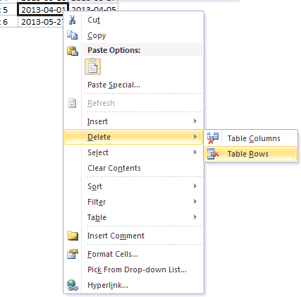
How to add or remove events
The events are in an excel defined table. You can add or remove rows by press with right mouse button oning on a cell and select Insert or Delete.
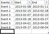
You can also add a blank row by selecting the last cell in the table.
Press Tab key.
You can move the table to any sheet you like.
Calendar category
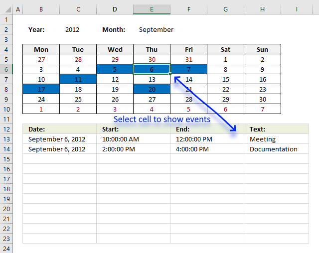
Table of Contents Excel monthly calendar - VBA Calendar Drop down lists Headers Calculating dates (formula) Conditional formatting Today Dates […]
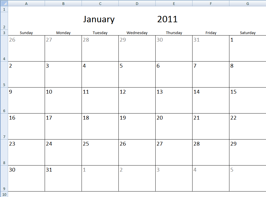
Table of Contents Monthly calendar template Monthly calendar template 2 Calendar - monthly view - Excel 365 Calendar - monthly […]
The image above demonstrates a calendar in Excel that allows you to: Add events. An event contains a date and […]
Excel categories
70 Responses to “Plot date ranges in a calendar”
Leave a Reply
How to comment
How to add a formula to your comment
<code>Insert your formula here.</code>
Convert less than and larger than signs
Use html character entities instead of less than and larger than signs.
< becomes < and > becomes >
How to add VBA code to your comment
[vb 1="vbnet" language=","]
Put your VBA code here.
[/vb]
How to add a picture to your comment:
Upload picture to postimage.org or imgur
Paste image link to your comment.
Hi.
So this is exactly what i am looking for to get my Staff Leave Calendar going except that my table (data sheet) is on another worksheet in the same workbook as the calendar. How can i amend the formula so that it works for me?
Lorne,
Conditional formatting can´t reference cells in other sheets. There is a workaround, use named ranges.
Hi,
thank you for the excellent article. I have only one question. Can I use the same method if the chart looks like this - https://www.freeimagehosting.net/d5b2k I want to add the months (in yellow) on top of the days and get rid of the red months.
I will appreciate any help. Thank you!
If you are interested, here are shorter alternate formulas for the first and last day of the month given the setup you posted above...
First Day: =1*(1&B2&B1)
Last Day: =(1&B2&B1)+31-DAY((1&B2&B1)+31)
Note: The parentheses are important and must remain as shown.
Rick Rothstein (MVP - Excel),
Thanks! Of course I am interested.
[...] on Jul.27, 2012. Email This article to a Friend I have created a new version of Visualize date ranges in a calendar. This excel file let´s you enter names and date ranges (A20:G33). Duplicate names are allowed. [...]
Hi,
There are several bugs in your calendar. The dates are not quite right for 2013, and I think this is because of the parameter chosen in the Weekday function.
Also, when the month starts on a Sunday, it drops down a line. I tried to fix this by changing the functions but then the Sunday was blanked and I didn't have time to unravel your conditional formatting.
regardless, this is very useful for me so thanks
Peter
Peter Clark,
thanks!
There are several bugs in your calendar. The dates are not quite right for 2013, and I think this is because of the parameter chosen in the Weekday function.
Corrected!
Also, when the month starts on a Sunday, it drops down a line.
I am not seeing this on my sheet.
Thanks for commenting!
Hi.
I have a worksheet that generates a schedule of milestone dates via formula after I type in one date. I use your calendars on different worksheets and I pull in the dates from my main sheet to insert into the table that you use to drive the calendars (only I have the start and end date the same since they are milestones-- only one day is highlighted on the calendar, not a range of days.) I then use Excel's camera utility to take an image of the calendar and put it on my main screen next to the generated dates.
The problem I'm having is when I create a second set of worksheets in the same workbook, the new calendars still want to show the values that were on the first set of worksheets, even though I've changed the pointers so they point to the dates on the new main sheet. Example: on the first set that worked-- the formula for the first start date in your calendar's table is:
='Nov 2013 Schedule Calculator'!E3
On my new set, the formula for the first start date in your calendar's table is:
='Aug 2013 Schedule Calculator'!E3
So the dates in the table are correct-- but the calendar seems to be getting its instructions on what to highlight from elsewhere.
How do I adjust this?
G. Cooley,
1. Select the picture in the second set of worksheets
2. Change the cell reference in the formula bar
3. Press Enter
Oscar-- thanks, that fixed it. This is great software.
I just have one last question. I did change the color from the gray to red so it stands out, and I'm using the same start and end date because I'm showing milestones, not ranges. It works fine, but I have a date-- Sept 4, 2013. It shows up in red on Sept 4, but it also shows up in as the red 4 in the bottom of the August block (in the area that is supposed to be white-one-white). Do you know what is causing that?
G. Cooley
Oscar: I think I may have figured this out. On your rule for formula IF(MONTH (J24)8,1,0) for August, you have the Format set to white lettering on a NO BACKGROUND. All your other conditional formatting rules like this have the format set to white lettering on a WHITE background. I changed it and this seems to have fixed the problem. (without this fix, if you have days in the table in that first week of September, they show up at the bottom of the August month-- in that row that is supposed to be white on white.
G. Cooley
Please group Name in row date ?
Jose,
Can you explain in greater detail?
I've been looking for something like this, but need to make a change. Currently if a name has two or more start and end dates in a the same month, each entry appears on a different row. I would like each name to appear only once, but all their dates from that month to appear on the calendar. Do you think this is possible? Thanks
Hi Oscar, thanks for this solution. Unfortunately my dates are not unique values, so the formula always pulls the smallest campaign name instead of the next campaign name, i.e. if the first 3 entries (James, James and Robert) all start on the same day, the calendar would show me 3 x James instead of James, James, Robert. Any idea on how to fix this? I assume I need to get rid of the SMALL formula but I can't quite get it to work. Any hints are welcome!
Am having a probem when it come with different names having the same dates,if 3 entries (James,Michael and Robert) all start on the same day, the calendar would show me 3 x James instead of James, Michael, Robert. Any idea on how to fix this?
Easiest way to resolve this is to use employee ID number or a unique identifier, thats what I've done
We are using your calendar for our machining work centers. One question though, is there a way to have multiple tabs (example, one tab would be grinding, one tab would be machining etc...)
I tried just copying the tab, but that doesn't seem to work.
Thanks,
Rob
Robert,
is there a way to have multiple tabs (example, one tab would be grinding, one tab would be machining
Yes!
1. Copy sheet
2. Select the new sheet
3. Find out the new table name (Select a cell in the table and press with left mouse button on tab "Design")
4. Change this conditional formatting formula, replace Table1 with the new table name (Table2):
=IF(B6="",FALSE,SUMPRODUCT((B6>=INDIRECT("Table1[Start]"))*(B6<=INDIRECT("Table1[End]")))) to =IF(B6="",FALSE,SUMPRODUCT((B6>=INDIRECT("Table2[Start]"))*(B6<=INDIRECT("Table2[End]"))))
Hi Oscar,
How can we add more than 13 names to be marked in the calendar?
I have an excel were I register the rented cars of a company and I want to mark the days the cars are rented in the calendar, I tried to add more rows and changed the formula to contain the rows that are being calculated but it doesnt seem to work.
Thank you
[…] run into a glitch with conditional formatting on a date range visualization spreadsheet I got from Visualize date ranges in a calendar part 2 | Get Digital Help - Microsoft Excel resource . I took the existing conditional format referencing green date ranges and modified it to add […]
Hi
This is really great thank you! It almost does exactly what I want/need.
The thing I'd love to be able to do is to start part way through one year, and end part way through the next - eg Start Oct 2014 and end the table at Sep 2015.
I've tried playing around with your sheet and I just cannot get it to do that.
For example how is your "invisible date" formula working out the month? It appears it can't be taking the letters "Jan" from A3, because if I simply change those to "Dec" then it still highlights the dates as though they are January.
How could I achieve what I want and have the table denoting the end of one year and the beginning of another?
Thanks again and all the best.
Hi,
I am using your formula, but instead of having the months downwards in colums I have an endless series.
It works, but for some reason it does not highlight the first day of some of the data range (two first ranges are not showing first date while third range works perfectly).
I have checked the invisible dates and they are correct. Do you have any idea as the reason why I am having this issue?
Cheers,
Jorunn
Hi again,
I figured it out. I used time in the date range (03.04.2015 06:00).
Do you know if there is a way wich makes you able to include the time without the effecting the vizualization?
Cheers
Jo,
Try this:
CF formula highlighting green cells:
=SUMPRODUCT((B3<=INT($I$20:$I$26))*(B3>=INT($E$20:$E$26)))=1
CF formula highlighting red cells:
=SUMPRODUCT((B3<=INT($I$20:$I$26))*(B3>=INT($E$20:$E$26)))>1
Many thanks for this, solved a problem I have been working on for a while. Is there any way of combining this conditional formating with another formula so that the cells are only formated if there is a certain name in the first column of the date ranges. I would like to format the dates with different colours for different people.
Many thanks
Hello,
Did you find a solution to this?
Hi,
Trying to get this to work, can't see where I am going wrong, changing the month increases the days to number of days in the year, if I put 2015 in the year I get 42005 in D1. Is something formatted wrong, can't see any formula errors.
Cheers
Simeon
Sorry sorted formats working now.
Ta!
Your calendar is exactly what I was looking for. My names and dates, however, are in a different tab and I cannot make it work. For example, this is one of the formulas reading from a tab called Pipeline. Any ideas on how to fix this?
=IFERROR(INDEX(Pipeline!$I$20:$I$1000, SMALL(IF((Pipeline!$D$20:$D$1000=$D$1),MATCH(Pipeline!$D$20:$D$1000,Pipeline!$D$20:$D$1000,0),""),ROW(A1))),"")
Is it possible to display Event name in calendar instead of highlight or first three letters of event
Great job on this. 2 quick questions.
1. Is there a way to make each event a different color?
2. Is there a way to make it so that if 2 event dates overlap that it makes the overlapping calendar dates highlighted red?
I will dig into it and figure it out but just thought you may have a quick answer.
Thanks!
I have the same question. Please let me know if you have figured this out.
Thanks,
Hossein.
Hi, this is the closest thing I have found to what I am looking for, however, it's not quite there.
I am essentially trying to create something very similar for tracking time off, but these are the following modifications I need:
1) The names starting in cell A5 would need to be fixed. So, essentially I want each name to appear only once and I would like to see all of their dates for that month appear in the calendar
2) The formula would need to take into consideration time splitting. So for example, if employee1 takes time off between July 1-5th and then again between July 25-27th, then I would like to see these cells in the calendar highlighted.
I would be so grateful if someone could provide a solution. I have seriously been searching for a solution on and off for the past 2 months and have come up with nothing yet.
Thanks!
Caroline,
1, How is your data arranged? Name and then a single date in each cell or multiple date ranges?
Hi,
Thanks for the formula this is almost what I was looking for, but is there a way to show the name of the person that has the range in the calendar?
So in the calendar the days 1 though 5 of February will have the name Theodor in the cells and so on?
Good afternoon,
I really like the calendar but I have few questions.
When I put multiple entry and dates overlap, some entry won't appears on the list.
Is there a way to make it indexed without the red highlight. Just have a list of all events and highlight the dates as well
Thank you
Eric
Can you provide some date examples where the entries won't appear?
Hi Oscar!
This is so close to what I am looking for, I wonder if you can help me with a couple of improvements:
- The conditional formatting shading fields where leave is taken to not just show shading but "A" in cell (meaning: Annual - eventually we would be looking to include additional leave types such as maternity leave, long service leave etc)
- At the end of the table, to count number of days leave taken for the view period
- Leave dates exclude public holiday and weekends?
TT,
The conditional formatting shading fields where leave is taken to not just show shading but "A" in cell (meaning: Annual - eventually we would be looking to include additional leave types such as maternity leave, long service leave etc)
- At the end of the table, to count number of days leave taken for the view period
I hope this is what you are looking for? See picture below.
Visualize-overlapping-date-ranges-part-2-version-TT.xlsx
Leave dates exclude public holiday and weekends?
The count excludes weekend but not public holidays.
Hi Oscar!
Thats so amazing! however when I tweak your sample (eg. I slot in my employee IDs and dates, the "A" coding disappear?
I've set it up so that all values are in single fields (non-merged fields), seems like when I unmerge fields and double check formulas, the "A" coding part of the formula breaks?
I also put the list of leave to the right of the calendar (as i'd like to format this template so that other departments can use it regardless of number of employees they have (eg. 5 or 100)
Can you tell me if I'm doing something wrong?
Also employee listing in column A is static as managers want to see out of those under their care who is taking leave and who is not
TT
however when I tweak your sample (eg. I slot in my employee IDs and dates, the "A" coding disappear?
Make sure the cell references point to the right cell ranges.
Hi Oscar,
This is a solution that I have been searching for! I followed your instructions and opened the document associated with the lesson and noticed in both that the Red Conditional formatting formula applied to cell range B5:AF17 yields an error stating that the formula is missing a parenthesis--) or (.
I've parsed out the formula in excel and double checked with no avail.
Am I missing a step here?
Resolved! We were able to parse out the formula this way
in any cell (for this we chose AI21) entered the following formula: =IF((INDEX($B$20:$B$33, SMALL(IF($A5=$A$20:$A$33, MATCH(ROW($B$20:$B$33), ROW($B$20:$B$33)), ""), COUNTIF($A$5:$A5, $A5)))=B$4)), SUMPRODUCT(($B$20:$B$33=B$4))>1, FALSE)
then set a conditional format to:
=IF( ( U26 =B$4)), SUMPRODUCT(($B$20:$B$33=B$4))>1, FALSE )
Everything worked.
April
I am happy you got it working.
when you set event1 date 1.1.2013 to 31.12.2013, you can see
august has a problem with coloring.
Hi Oscar,
I am using your visualize overlapping date range part 2 template and when i am trying to change the range from B33 to B41 the template stops working I mean it does not work. Please help.
I have the above shown Leave Matrix which shows the employees and their Leaves for the month/year. How can i Generate the records for them that you are showing as manual entries ?
Rehan Memo,
great question! See this article:
https://www.get-digital-help.com/get-date-ranges-from-a-schedule/
Is it possible to set conditional formatting to only highlight dates that overlap if there are more than 3 people for example that want vacation at the same time for overlapping dates?
Michelle,
Yes, it is possible.
You need to change two CF formulas.
Red:
=SUMPRODUCT((B3=$E$19:$E$26))>3
Green:
=(SUMPRODUCT((B3=$E$19:$E$26))<=3)*(SUMPRODUCT((B3=$E$19:$E$26))>=1)
Get the workbook:
Plot-date-ranges-in-a-worksheet-3-or-more.xlsx
Oscar,
I have the same issue as Simone from June 24 2013. I do not have unique start dates. I do have unique names. If I have James, Karl, and John with the same start date I receive three rows of James. Any solutions yet? I am using the TT version which is great. Thanks for your knowledge
Mark,
Thank you for telling me, I have made some changes to the TT workbook. Let me know if this is what you are looking for.
Visualize-overlapping-date-ranges-part-2-version-TT1.xlsx
Oscar,
You're a genius. Thank You!
Mark,
you are welcome!
This file is amazing, it is exactly what I am searching for. But can't understand why when I double press with left mouse button on any value (name or "A" in the calendar) data dissapier...Also I tried to add more rows and changed the formula to contain the rows that are being calculated but it doesnt seem to work..
I'm looking for a template that will allow me to create a calendar reflecting a year in columns (by week), and scheduled tasks by individuals. The tasks are shared, so there are multiple people working on a single task, and it should be filterable by task name (or number).
Can this be done?
Hi! For some reason no numbers will show in my row 4, and both "TRUE" and "FALSE" are showing. I am copying and pasting formulas, but I am using Google Sheets not Excel (which might be an issue).
I was also hoping to find out if I could add more columns as I need to show both a campaign, and a car number in certain locations based on the calendar year. It has been complex since there are many variables to show at once.
Hoping you can help!
Thank you.
This is great. I will preface this comment by stating I am attempting to use Google Sheets not Excel. Unfortunately nothing shows in row "4." Along with this both "FALSE" and "TRUE" are appearing in my cells. If possible I would love to include a location dropdown along with car numbers at each given time. It's been a struggle creating and/or finding something to show three variables at any given time throughout the year (Campaign, Car #, and Location). Thank you!
Hello,
This calendar is amazing. I'm trying to make one change. I would like different employees to show up as different colors. Any idea how I can do that? TIA.
Hi .... Excel Developer
This is A good aplication but there is a bugs i found..
If we Summit the Same date and same year in table, the result is not right, ..
Can you email to me, the file if you done to Fixed.
Thank you So much,...
From Indonesia
I need to highlight Saturdays and Sundays with a different color. Can someone assist here?
BUENAS NOCHES Y MUCHAS GRACIAS, ME AYUDO MUCHO ESTA INFORMACION SOBRE PERSONALIZAR LA PLANTILLA DE CALELDARIO.
GRACIAS,..!!
Google translate: GOOD NIGHT AND THANK YOU VERY MUCH, THIS INFORMATION ON CUSTOMIZING THE CALENDAR TEMPLATE HELPED ME A LOT. THANK YOU,..!!
In first section not ; but ,
Hi Oscar, this is so close to what I'm looking for! What I need is something that will plot the date range across the full year (not just 1 month at a time), is there an easy way to change the formula so it shows Jan1-Dec31 across the columns?
Good afternoon, this is amazing!
Is it possible to highlight the a particular date range (as above in green) but based on a name in another column?
Thanks a lot!
I want to add “Leave type” column in the table and apply different colours for each of these, how can i apply that changes in formatting condition formula? For example if sick leave blue, vacation green
Assistance request. I am using this solution to create a travel calendar for myself. this is working great to show the dates that I am traveling and also where I have overlapping travel dates. What I am trying to do is add a check to the conditional formatting that looks at my field Table1 Booked. So my field on my Table1 called Booked is yes, then I want to indicate that somehow. Maybe change the formatting color. I am using this version for conditional formatting. I am sure this is a simple add but I just can't figure it out.
=(INDEX(INDIRECT("Table1[Start]"), SMALL(IF($A5=INDIRECT("Table1[Name]"), MATCH(ROW(INDIRECT("Table1[Start]")), ROW(INDIRECT("Table1[Start]"))), ""), COUNTIF($A$5:$A5, $A5)))=B$4))