Cleaning Up Excel Worksheets: Eliminating Blank Cells, Rows, and Errors
![]()
In this blog post I will demonstrate methods on how to find, select, and deleting blank cells and errors.
Why clean up a data set?
- Errors and inconsistencies can impact analysis.
- Improves filtering and sorting which makes it easier to organize and analyze data.
- Formulas and functions may break meaning they return an error value.
- An error value or blank may break visualization tools like charts and graphs.
- Unnecessary data takes storage space which increases file size.
- Blanks may cause incorrect calculations if included.
- Easier to quickly select data if blanks and empty rows are removed.
What is a blank cell?
A blank refers to a cell that is completely empty, note that a cell may look empty but may contains invalid characters or a space character that is not visible.
What is a blank row?
All cells are completely empty. A list or data set is non-contiguous if a blank row exists meaning there are data that are not adjacent to each other. This makes it impossible to select the entire data set using the short cut keys CTRL + A.
Table of Contents
- Remove blank cells - formula
- Remove blank cells [keyboard shortcut F5]
- Remove blank rows - formula
- How to delete empty rows - advanced filter
- Delete blanks and errors in a list
- How to find errors in a worksheet
- How to find blank cells
- How to quickly select blank cells
- Identify all characters in a cell value
- Identify all characters in a cell value - Excel 365
- How to remove unwanted characters in a cell
- How to select cells containing data
- How to select a non contiguous range
- How to improve worksheet readability in Excel
- How to quickly select a cell range
- How to quickly select a named range or an Excel table
- How to quickly select a contiguous cell range
- How to name a cell range
- How to link to a specific cell range
- Different ways to delete a cell value
- Different ways to delete an entire cell
- Select and delete blank cells
- Select and delete formulas returning a given condition
- Macro deletes formulas returning a blank
- Macro deletes entire row if the formula returns blanks
- Get excel *.xlsm file
1. Remove blank cells - formula
![]()
Column B is the list with random blank cells. Column D is the list without the blank cells.
Excel 365 formula in cell D3:
The FILTER function spills values automatically to cells below, the #NUM error shown in the image above is not returned if you use the FILTER function.
The following array formula in cell D3 is for versions before Excel 365:
This older formula returns a #NUM error when there are no more values to display. Section 1.3 below provides a solution to this problem.
1.1 How to enter an array formula
Excel 365 users can skip these steps, a dynamic array formula in Excel 365 is entered as a regular formula by pressing the Enter key.
- Copy (Ctrl + c) and paste (Ctrl + v) array formula into formula bar. See picture below.
- Press and hold Ctrl + Shift.
- Press Enter once.
- Release all keys.

1.2 How to copy array formula - older versions
Excel 365 users can ignore this.
- Copy (Ctrl + c) cell D3
- Paste (Ctrl + v) array formula on cell range D3:D8
1.3 Remove #num errors (excel 2007) - older versions
Excel 365 users can ignore this.
When you run out of values to show, the array formula above returns #NUM! errors. You can avoid this if you use the IFERROR function, however use it with great caution. It not only finds #NUM! errors but all errors. So if you formula or cells contain an error you won't see it, the IFERROR function removes that error too.
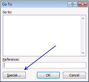
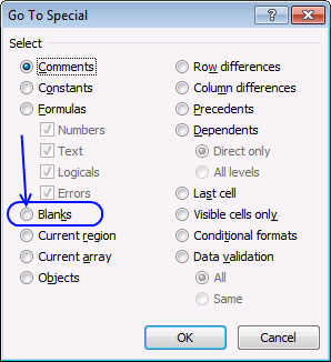
2. Remove blank cells [keyboard shortcut F5]
![]()
The image above shows random cell values in column B, follow these simple steps to remove blank cells in column B.
- Select range B2:B12.
- Press F5 and a dialog box appears.

- Press with left mouse button on "Special..." button.

- Press with left mouse button on radio button "Blanks".
- Press with left mouse button on OK button. The image below shows that the cell range selection changed, now only blank cells are selected.
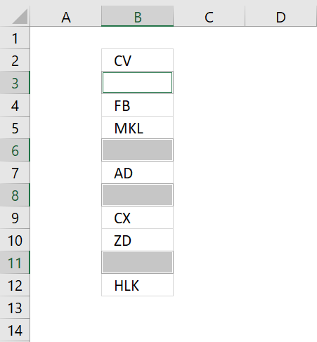
- Press with right mouse button on on one of the selected blank cells and a context menu appears, select "Delete..".

- Another dialog box appears, press with left mouse button on "Shift cells up".

"Shift cells up" will delete selected blank cells and move non empty cells up. This step will mess up your dataset if you have values arranged as records.
"Entire row" will delete row 3, 6, 8 and 11 in image above. If you have data on these rows they will be deleted as well. - Press with left mouse button on OK button.

![]()
The image above shows that blank cells are now deleted.
3. Remove blank rows - formula
![]()
This example demonstrates how to filter out blank rows meaning both cells on the same row must be empty.
Excel 365 dynamic array formula in cell E1:
The FILTER function returns values automatically to cells below, this is called spilling by Microsoft.
Array formula in cell E2 is for earlier versions:
3.1 How to create an array formula
Excel 365 users can ignore these steps, a dynamic array formula in Excel 365 is entered as a regular formula by pressing the Enter key.
- Select cell E2
- Paste formula
- Press and hold Ctrl + Shift
- Press Enter
3.2 How to copy array formula
Excel 365 users can skip these steps.
- Select cell E2
- Copy cell (Ctrl +c)
- Select cell range E2:E10
- Paste
4. How to delete empty rows - advanced filter
![]()
I highly recommend you keep the original data and only copy the data excluding blank rows and paste to a new worksheet.
Let me explain why, if you by accident delete rows partially empty and don't notice it or use a macro that you can't undo, then that data is gone.
![]()
I am going to use the Advanced Filter to hide blank rows, in order to do that I need to add a criteria range.
The criteria range consists of the table header names and the criteria below the header names, see cell range B2:D5 in the picture above.
Make sure the criteria header names are identical to the table header names.
The criteria are <> meaning not equal to nothing. They are on a row each so at least one condition must be true (OR logic) to filter a row.
It is now time to start the Advanced Filter, go to tab "Data" on the ribbon. Press with mouse on the "Advanced" button.
![]()
The "Advanced Filter" dialog box appears.
![]()
Select the criteria range and the list range, then press with left mouse button on OK button.
![]()
Select and copy cell range B7:D17 and paste to a new worksheet.
![]()
If you paste the data next to your original table remember to clear the filter so you can see all the rows.
![]()
5. Delete blanks and errors in a list
![]()
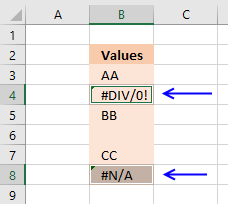
What are error values?
An error value is returned when something is wrong, it may be a formula that contains an error, a function with missing parameters or a misspelled function etc, invalid argument, or wrong data type.
Here are a few common errors in Excel:
- #NULL error - This error occurs most often if you by mistake use a space character in a formula where it shouldn't be. Excel interprets a space character as an intersection operator. If the ranges don't intersect an #NULL error is returned. The #NULL! error occurs when a formula attempts to calculate the intersection of two ranges that do not actually intersect. This can happen when the wrong range operator is used in the formula, or when the intersection operator (represented by a space character) is used between two ranges that do not overlap. To fix this error double check that the ranges referenced in the formula that use the intersection operator actually have cells in common.
- #SPILL error - The #SPILL! error occurs only in version Excel 365 and is caused by a dynamic array being to large, meaning there are cells below and/or to the right that are not empty. This prevents the dynamic array formula expanding into new empty cells.
- #DIV/0 error - This error happens if you try to divide a number by 0 (zero) or a value that equates to zero which is not possible mathematically. Use the "Evaluate formula" tool to pinpoint the exact location in the formula where this error occurs. The "Evaluate formula" tool is located on the "Formulas" tab on the ribbon. Select the cell containing the #DIV/0 error and then press with left mouse button on the "Evaluate formula button".
- #VALUE error - The #VALUE error occurs when a formula has a value that is of the wrong data type. Such as text where a number is expected or when dates are evaluated as text.
- #REF error - The #REF error happens when a cell reference is invalid. This can happen if a cell is deleted that is referenced by a formula.
- #NAME error - The #NAME error happens if you misspelled a function or a named range.
- #NUM error - The #NUM error shows up when you try to use invalid numeric values in formulas, like square root of a negative number.
- #N/A error - The #N/A error happens when a value is not available for a formula or found in a given cell range, for example in the VLOOKUP or MATCH functions.
- #GETTING_DATA error - The #GETTING_DATA error shows while external sources are loading, this can indicate a delay in fetching the data or that the external source is unavailable right now.
The formula deletes blank cells and cells with errors. It doesn't matter if the cells contain numbers or text, they all will be presented in a new column.
Excel 365 formula in cell D3:
Array formula in cell D3:
5.1 How to create an array formula
- Copy (Ctrl + c) and paste (Ctrl + v) array formula into formula bar. See picture below.
- Press and hold Ctrl + Shift.
- Press Enter once.
- Release all keys.
5.2 How to copy array formula
- Copy (Ctrl + c) cell D3
- Paste (Ctrl + v) array formula on cell range D3:D11
5.3 Explaining formula in cell D3
Step 1 - Identify blank cells
The ISBLANK function returns TRUE if cell is blank (empty) and FALSE if not.
ISBLANK($B$3:$B$20)
returns {FALSE; FALSE;... ; FALSE}
Step 2 - Identify errors
The ISERROR function returns TRUE if cell contains an error and FALSE if not.
ISERROR($B$3:$B$20) returns {FALSE; FALSE; ... ; TRUE}
Step 3 - Add arrays
If at least one of the boolean values is TRUE then the result must be TRUE, addition is what we need to use.
| Boolean | Boolean | Multiply | Add |
| FALSE | FALSE | 0 (zero) | 0 (zero) |
| FALSE | TRUE | 0 (zero) | 1 |
| TRUE | TRUE | 1 | 2 |
ISBLANK($B$3:$B$20)+ISERROR($B$3:$B$20) returns {0; 0; ... ; 1}.
Step 4 - Convert array to row numbers
The IF function lets you use a logical expression to determine which value (argument) to return.
IF(ISBLANK($B$3:$B$20)+ISERROR($B$3:$B$20), "", MATCH(ROW($B$3:$B$20),ROW($B$3:$B$20)))
returns {1;2;... ;""}
Step 5 - Get k-th smallest row number
To be able to return a single value from the array we need to use the SMALL function to extract a single row number. The second argument in the SMALL function uses the ROWS function with an expanding cell reference to extract a new value in each cell.
SMALL(IF(ISBLANK($B$3:$B$20)+ISERROR($B$3:$B$20), "", MATCH(ROW($B$3:$B$20),ROW($B$3:$B$20))), ROWS($A$1:A1))
returns 1.
Step 6 - Return value based on row number
The INDEX function returns a value from a cell range based on a row and column number, our cell range is a single column so we need to only specify a row number in order to get the correct value.
INDEX($B$3:$B$20, SMALL(IF(ISBLANK($B$3:$B$20)+ISERROR($B$3:$B$20), "", MATCH(ROW($B$3:$B$20),ROW($B$3:$B$20))), ROWS($A$1:A1)))
returns 2 in cell D3.
5.4 Get excel *.xls
6. How to find errors in a worksheet
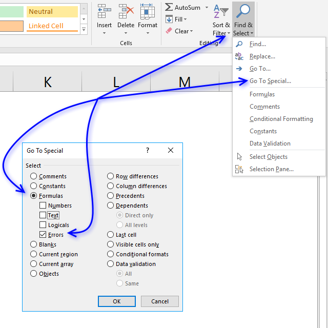
Excel has great built-in features, the following one lets you search an entire worksheet for formulas that return an error.
Instructions:
- Go to "Home" tab

- Press with left mouse button on "Find & Select"
- Press with left mouse button on "Go to Special..."
- Press with left mouse button on "Formulas"
- Enable "Errors"

- Press with left mouse button on ok!
If any formula errors exist, they are now selected. The picture below demonstrates error cells being selected.
7. How to find blank cells
![]()
In this article, I am going to show you two ways on how to find blank cells. Both techniques are quick and easy.
The first one allows you to find each blank one by one. The picture above shows you the first example, I want to find blanks in column D.
- Select the first value in the column you want to search.
- Press and hold CTRL key.
- Press down arrow key once.
 +
+ ![]()
This will move the selection right above the first blank cell in the same column, see picture below.
![]()
Press down arrow key twice still holding the CTRL key will move the selection to the next blank cell in your worksheet.
The second way lets you create a list of all blanks in your worksheet.
![]()
- Press with mouse on the first value in the column, then press CTRL + SHIFT + END keys to select all values including blanks in the column.
I have selected cell range D2:D355, see picture above. - Press CTRL + H to open the "Find and Replace" dialog box.
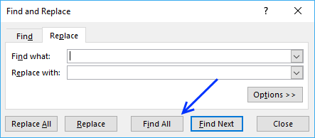
- Don't enter anything, simply press with left mouse button on the "Find All" button.
The dialog box now shows all blank cells with their location, see picture below.
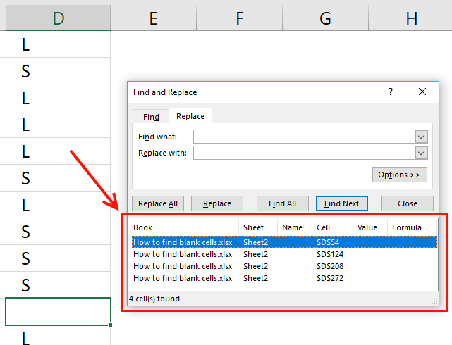
Press with mouse on a row in the dialog box to instantly move to and select that blank cell.
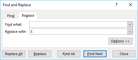
Tip! Use the "Find and Replace" dialog box to fill blank cells with a value. The example below replaces all blank cells with S.
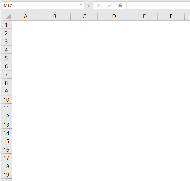
8. How to quickly select blank cells
![]()
In this smaller example, column D (Category) has empty cells, shown in the picture above. If your column contains thousands of cells manually selecting those cells, one by one will be tedious and time-consuming.
Luckily there is a wonderful trick that will save us lots of time, the following steps demonstrate how to select blank cells in a cell range:
- Select cell range D3:D15.
- Press function key F5 on your keyboard.

- Press with mouse on button "Special...".
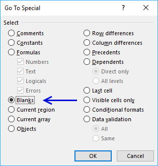
- Select "Blanks"
- Press with left mouse button on OK button
![]()
The picture above shows all blank cells selected in cell range D3:D15.
Read the following article on how to enter a formula or data in all selected cells:
Recommended articles
VBA Macro
The following macro will be handy if you often find yourself often selecting blank cells in a specific cell range.
Sub Macro1()
Selection.SpecialCells(xlCellTypeBlanks).Select
End Sub
Where to copy code?
- Copy above macro
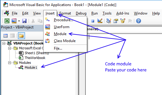
- Go to VBA Editor (Alt+F11)
- Press with left mouse button on "Insert" on the top menu
- Press with left mouse button on "Module" to insert a module to your workbook
- Paste code into the code window
- Exit VBA Editor and return to Excel (Alt+Q)
Save your workbook
To be able to use the macro next time you open your workbook you need to save the workbook as a macro-enabled workbook.
- Press with left mouse button on "File" on the menu, or if you have an earlier version of Excel, press with left mouse button on the office button.
- Press with left mouse button on "Save As"
- Press with left mouse button on file extension drop-down list
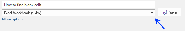
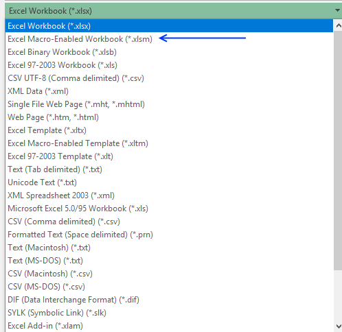
- Change the file extension to "Excel Macro-Enabled Workbook (*.xlsm)".
Tip! Link the macro to a button on the "Quick Access Toolbar" to have it freely available when needed.
9. Identify all characters in a cell value
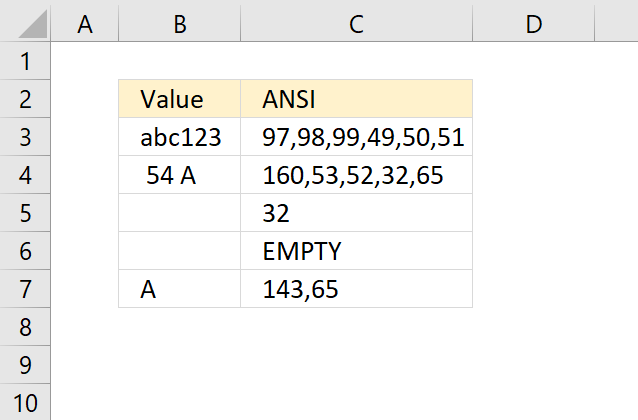
Sometimes when you sort values you get unexpected results, the cause is probably unwanted characters in a cell.
The same thing may happen if you try to trim blanks in a cell value and it fails to remove the character that looks like the space character.
The TRIM function removes only ANSI character 32, however, the HTML blank character number 160 is not removed by TRIM.
The following array formula demonstrated in cell C3 in the picture above will convert each character in a cell value to its corresponding ANSI number (PC).
This will make it easier for you to see all the characters that cause problems. Cell B3 contains only letters and numbers, nothing weird.
Cell B5 contains a single space character, code 32. However, cell B4 contains an HTML character that looks like a space character. Cell B7 also has a weird space character, code 143.
As you can see the formula above assists you in finding weird characters.
Explaining formula in cell C3
Step 1 - Count characters
LEN(B3)
Step 2 - Create cell reference to a cell
INDEX($A$1:$A$1000, LEN(B3))
Step 3 - Create a cell reference to a cell range
The INDEX function and the LEN function allows you to create a cell reference with as many rows as there are characters in cell C3.
$A$1:INDEX($A$1:$A$1000, LEN(B3)) becomes $A$1:INDEX($A$1:$A$1000, 6) and returns $A$1:$A$6.
Step 4 - Create a sequential list of numbers from 1 to n
The ROW function then creates an array from 1 to the number of characters in cell C3.
ROW($A$1:INDEX($A$1:$A$1000, LEN(B3))) becomes ROW($A$1:$A$6) and returns {1;2;... ;6}
Step 5 - Split characters into an array
Now it is time for the MID function to split each character in cell C3 to an array.
MID(B3, ROW($A$1:INDEX($A$1:$A$1000, LEN(B3))), 1) returns {"a";"b";"c";"1";"2";"3"}
Step 6 - Convert characters into ANSI numbers
The CODE function allows you to convert a character to ANSI code (PC). We are using an array so the function will convert all characters at the same time.
CODE(MID(B3, ROW($A$1:INDEX($A$1:$A$1000, LEN(B3))), 1))) returns {97;98;... ;51}.
Step 7 - Join values in the array
Lastly, the TEXTJOIN function concatenates all values in the array with the delimiting character , (comma).
TEXTJOIN(",", TRUE,CODE(MID(B3, ROW($A$1:INDEX($A$1:$A$1000, LEN(B3))), 1)))
returns 97,98,99,49,50,51 in cell C3.
Step 8 - Catch errors
IFERROR(TEXTJOIN(",", TRUE,CODE(MID(B3, ROW($A$1:INDEX($A$1:$A$1000, LEN(B3))), 1))), "EMPTY")
If the cell value is empty the formula returns #VALUE, the IFERROR function then displays "EMPTY".
ANSI table
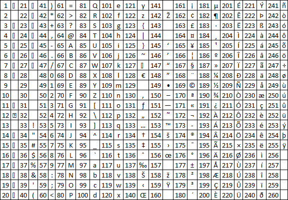
The picture above shows characters for number 1 to 255 (ANSI).
10. Identify all characters in a cell value - Excel 365
Excel 365 dynamic array formula in cell C3:
2.1 Explaining formula
Step 1 - Count characters
LEN(B3) returns 6.
Step 2 - Create a sequential list of numbers from 1 to n
SEQUENCE(LEN(B3)) returns {1;2;... ;6}
Step 3 - Split characters into an array
Now it is time for the MID function to split each character in cell C3 to an array.
MID(B3, SEQUENCE(LEN(B3)), 1) returns {"a";"b";"c";"1";"2";"3"}
Step 4 - Convert characters into ANSI numbers
The CODE function allows you to convert a character to ANSI code (PC). We are using an array so the function will convert all characters at the same time.
CODE(MID(B3, SEQUENCE(LEN(B3)), 1)) returns {97;98;... ;51}.
Step 5 - Join values in the array
Lastly, the TEXTJOIN function concatenates all values in the array with the delimiting character , (comma).
TEXTJOIN(",", TRUE,CODE(MID(B3, SEQUENCE(LEN(B3)), 1)))
returns 97,98,99,49,50,51 in cell C3.
Step 6 - Catch errors
IFERROR(TEXTJOIN(",", TRUE,CODE(MID(B3, SEQUENCE(LEN(B3)), 1))), "EMPTY")
If the cell value is empty the formula returns #VALUE, the IFERROR function then displays "EMPTY".
Get Excel *.xlsx file
Identify characters in a cell value.xlsx
11. How to remove unwanted characters in a cell
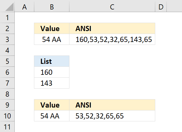
Cell B3 contains a few odd characters and the formula in C3 shows the ANSI equivalent of each character in B3. If you are interested in how I built the formula, read this: How to identify characters in a cell value
For example, 160 is an HTML space character that the TRIM and CLEAN function can't remove. You can remove a single character using the SUBSTITUTE function, however, if your cell contains multiple unwanted characters the following formula will remove specific characters.
Array formula in cell B10:
The characters I want to remove are in B6:B7 in ANSI code format. The formula in cell C10 shows that 160 and 143 are now gone in cell B10.
9.1 Explaining formula in cell B10
Step 1 - Count characters
LEN(B3)
Step 2 - Create a cell reference
INDEX($A$1:$A$1000, LEN(B3))
Step 3 - Create a cell range reference
The INDEX function and the LEN function allow you to create a cell reference containing as many rows as there are characters in cell B3.
$A$1:INDEX($A$1:$A$1000, LEN(B3)) returns $A$1:$A$7.
Step 4 - Create a sequential list of numbers from 1 to n
The ROW function then creates an array from 1 to the number of characters in cell C3.
ROW($A$1:INDEX($A$1:$A$1000, LEN(B3))) returns {1;2;3;4;5;6;7}
Step 5 - Split characters into an array
Now it is time for the MID function to split each character in cell C3 to an array.
MID(B3, ROW($A$1:INDEX($A$1:$A$1000, LEN(B3))), 1) returns {" ";"5";"4";" ";"A";"";"A"}
Step 6 - Convert characters to equivalent ANSI numbers
The CODE function allows you to convert a character to ANSI code (PC). We are using an array so the function will convert all characters at the same time.
CODE(MID(B3, ROW($A$1:INDEX($A$1:$A$1000, LEN(B3))), 1))
becomes
CODE({" ";"5";"4";" ";"A";"";"A"}) and returns {160;53;52;32;65;143;65}
Step 7 - Check ANSI numbers against list
The COUNTIF function counts how many times 160 and 143 are found in the array.
COUNTIF(B6:B7, CODE(MID(B3, ROW($A$1:INDEX($A$1:$A$1000, LEN(B3))), 1)))
returns {1;0;0;0;0;1;0}
Step 8 - Filter values
The IF function checks the logical expression and returns a blank value if TRUE and the character if FALSE. The IF function evaluates TRUE as 1 and FALSE as 0 (zero).
IF(COUNTIF(B6:B7, CODE(MID(B3, ROW($A$1:INDEX($A$1:$A$1000, LEN(B3))), 1))), "", MID(B3, ROW($A$1:INDEX($A$1:$A$1000, LEN(B3))), 1))
returns {"";"5";"4";" ";"A";"";"A"}.
Step 9 - Join characters
Lastly, the TEXTJOIN function concatenates the remaining characters in the array ignoring blank values.
TEXTJOIN(, TRUE, IF(COUNTIF(B6:B7, CODE(MID(B3, ROW($A$1:INDEX($A$1:$A$1000, LEN(B3))), 1))), "", MID(B3, ROW($A$1:INDEX($A$1:$A$1000, LEN(B3))), 1)))
returns 54 AA in cell B10.
Get Excel *.xlsx file
How to remove unwanted characters from cell value.xlsx
9.2 How to remove unwanted characters in a cell - Excel 365 formula
Excel 365 dynamic array formula in cell B10:
9.3 Explaining formula
Step 1 - Count characters
LEN(B3)
Step 2 - Create a sequential list from 1 to n
SEQUENCE(LEN(B3))
Step 3 - Split characters into an array
Now it is time for the MID function to split each character in cell C3 to an array.
returns {" ";"5";"4";" ";"A";"";"A"}
Step 4 - Convert characters to equivalent ANSI numbers
The CODE function allows you to convert a character to ANSI code (PC). We are using an array so the function will convert all characters at the same time.
CODE(MID(B3, SEQUENCE(LEN(B3)), 1))
returns {160;53;52;32;65;143;65}
Step 5 - Check ANSI numbers against list
The COUNTIF function counts how many times 160 and 143 are found in the array.
COUNTIF(B6:B7, CODE(MID(B3, SEQUENCE(LEN(B3)), 1)))
returns {1;0;0;0;0;1;0}
Step 6 - Filter values
The IF function checks the logical expression and returns a blank value if TRUE and the character if FALSE. The IF function evaluates TRUE as 1 and FALSE as 0 (zero).
IF(COUNTIF(B6:B7, CODE(MID(B3, SEQUENCE(LEN(B3)), 1))), "", MID(B3, SEQUENCE(LEN(B3)), 1))
returns {"";"5";"4";" ";"A";"";"A"}.
Step 7 - Join characters
The TEXTJOIN function concatenates the remaining characters in the array ignoring blank values.
TEXTJOIN(, TRUE, IF(COUNTIF(B6:B7, CODE(MID(B3, SEQUENCE(LEN(B3)), 1))), "", MID(B3, SEQUENCE(LEN(B3)), 1)))
returns 54 AA
Step 8 - Simplify formula
The LET function lets you name intermediate calculation results which can shorten formulas considerably and improve performance.
LET(name1, name_value1, calculation_or_name2, [name_value2, calculation_or_name3...])
TEXTJOIN(, TRUE, IF(COUNTIF(B6:B7, CODE(MID(B3, SEQUENCE(LEN(B3)), 1))), "", MID(B3, SEQUENCE(LEN(B3)), 1)))
has two repeating intermediate calculations bolded in the formula above:
MID(B3, SEQUENCE(LEN(B3)), 1) - x
I named it x.
LET(x,MID(B3, SEQUENCE(LEN(B3)),1),TEXTJOIN(,TRUE,IF(COUNTIF(B6:B7,CODE(x)),"",x)))
12. How to select cells with data
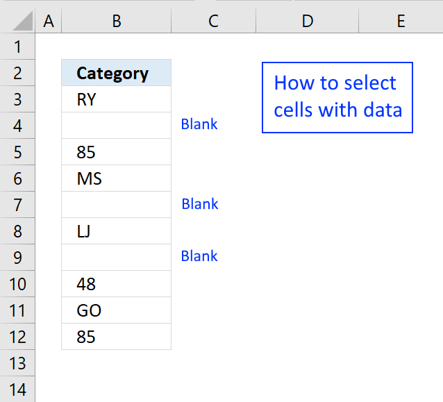
The picture above shows data in column B, some cells contain nothing, they are blank.
I will now go through the steps on how to select cells containing data excluding blank cells, formulas, and error values.
- Select cell B3
- Press CTRL + SHIFT + END keys to select all values including blanks.
- Press function key F5
- Press with left mouse button on "Special..." button located at the bottom left corner of the dialog box.
- Double press with left mouse button on "Constants"
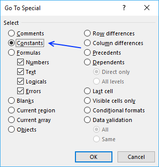
This will select all cells that contain numbers, text, boolean and error values.
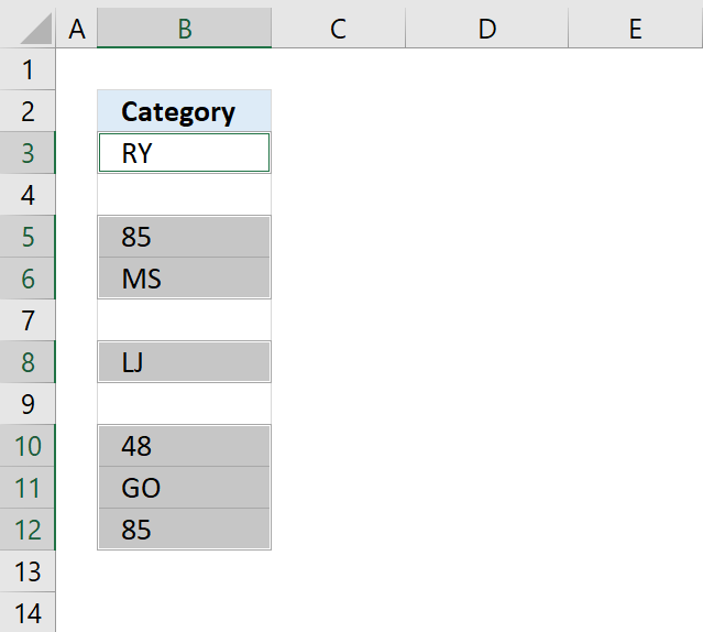
Note that cells containing a space character will be selected as well.
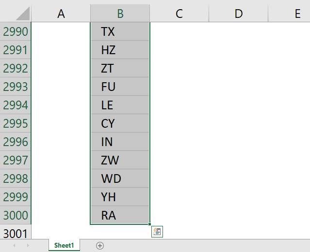
13. How to select a non contiguous range
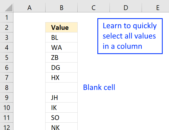
A non-contiguous list is a list with occasional blank cells and that makes it harder to select the entire cell range.
The picture above shows a part of a list that has 3000 values with occasional blanks. How do we quickly select the entire list?
The first thing that comes to mind is selecting this list using CTRL + SHIFT + DOWN ARROW but as you might know, the selection stops at every blank cell.
Here is how to select the entire list:
- Select cell B2
- Press CTRL + SHIFT + END
You have now selected the entire non-contiguous list.
VBA Macro
If you record a macro while pressing CTRL + SHIFT + END you get the following code:
Sub Macro1()
Range(Selection, ActiveCell.SpecialCells(xlLastCell)).Select
End Sub
Make sure you select the first value in the column before you run the macro.
Get Excel *.xlsm file
Select a non contiguous range.xlsm
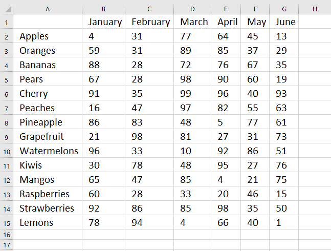
14. How to improve worksheet readability in Excel
How to make your worksheets useful?
Making your sheets easy to read is a fundamental approach of creating useful worksheets. Your message must be crystal clear, a misinterpreted sheet can be devastating. A sheet must be easy to read and follow.
Why create easy to read worksheets?
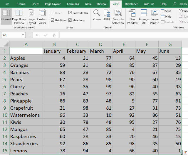
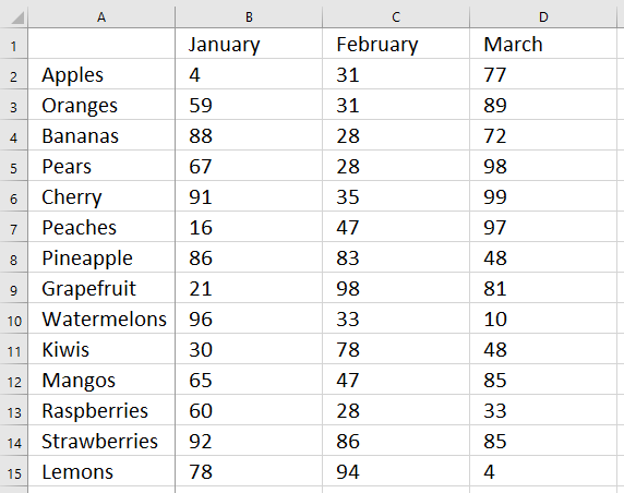
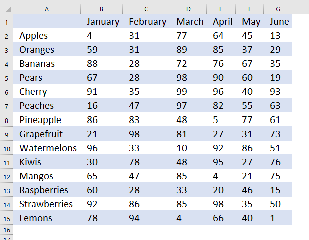
The above picture is an example of a simple sheet with some random numbers. It is really hard to follow let us say Kiwis monthly numbers to the right. Scrolling and larger columns is also a troublemaker for readers. Sheets printed out on paper has the same problem.
Worksheets must be easy to read in order to be useful.
What's on this section
- How to change the zoom level?
- How to change the Font size?
- How to create an indent?
- How to resize all cell column widths?
- How to lock first row and first column while scrolling?
- How to make two worksheets visible on the same screen?
- Create a chart
- Use sparklines to visualize data
14.1. How to change the zoom level?
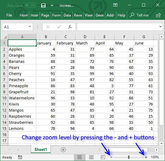
Use the zoom in and out buttons located at the bottom right of your Excel window to use your screen area more efficiently.
The "Zoom to Selection" tool located on tab "View" on the ribbon allows you to quickly zoom in to your selected cell range.
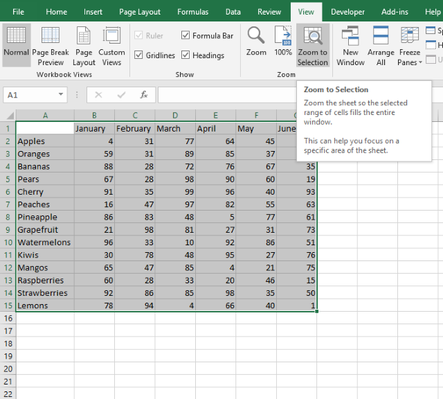
The "Zoom to Selection" tool is quicker than trying to use the + and - zoom buttons which are not that granular to make it a perfect fit.
The shortcut keys to zoom to selection is Alt + w + g. First press and release Alt then press and release w and lastly press and release g on your keyboard.
14.2. How to change the Font size
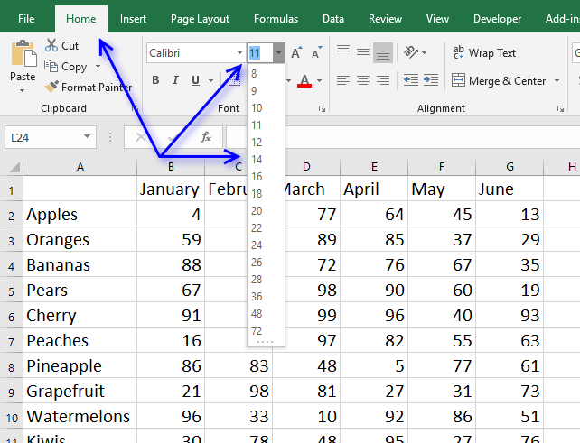
Increase the font size to make the text easier to read.
- Select the data.
- Go to tab "Home" on the ribbon.
- Press with left mouse button on the font size drop-down list.
- Select a size.
14.3. Create an indent
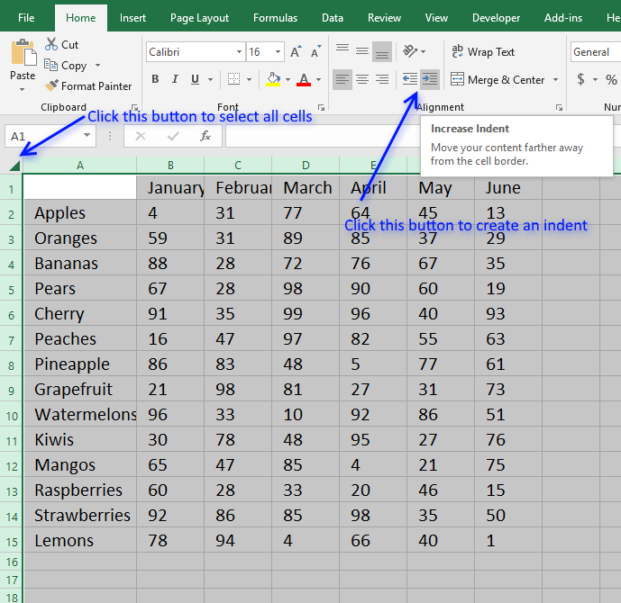
Follow these steps to add an indent to all cells on the worksheet:
- Press with left mouse button on the upper left button of your cell grid to select all cells.
- Press with mouse on the indent button on tab "Home" on the ribbon.
This moves all values to the right making the worksheet more visually appealing.
14.4. How to resize all cell column widths?
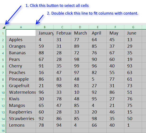
The picture below shows columns with variable width based on cell contents.
It is also visually appealing to have the same width of all columns. Follow these steps to make all columns on your worksheet equally large.
- Press with left mouse button on the upper left button of your cell grid to select all cells.
- Press and hold with left mouse button on the column line with the largest width to see it's column width.
The picture below demonstrates the line to press and hold in order to see the width of column A. - Now press and hold on a column line of a smaller column.
- Drag to the right to increase the column width, make it as big as the largest column.
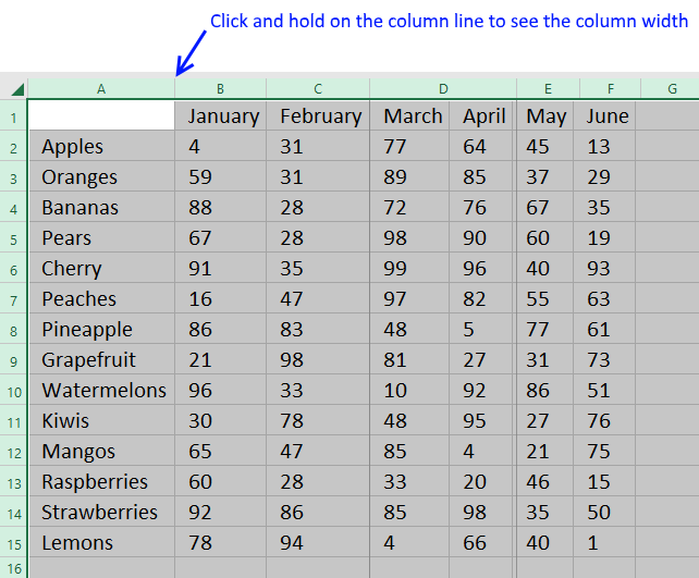
Voila! All columns now have the same width as the largest column on your worksheet.
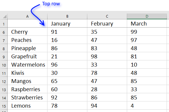
14.5. How to lock first row and first column while scrolling?
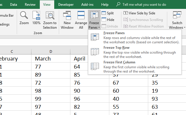
Excel allows you to keep specific rows and columns visible while the remaining worksheet scrolls. This makes it easier to read huge data tables, you always have the headers visible.
- Go to tab "View" on the ribbon.
- Press with left mouse button on "Freeze Panes" button
- You now have three options:
- Freeze rows and columns based on the selection.
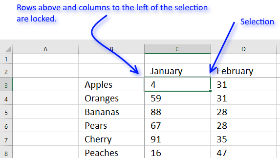
- Freeze top row.
- Freeze the first column.
- Freeze rows and columns based on the selection.
There is a thin line between the frozen column or row and the rest of the worksheet.
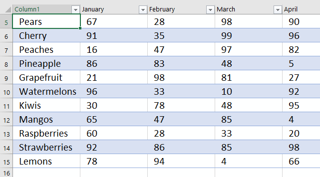
You also have the option to convert the data set to an Excel defined table, this will automatically keep the headers visible while scrolling the data. The image above shows you an Excel defined table.
- Press with left mouse button on a cell in the data set you want to convert to an Excel defined table
- Press CTRL + T
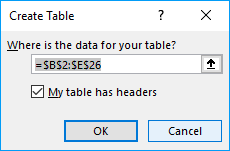
- Select checkbox if the table contains headers.
- Press with left mouse button on OK button.
14.6. How to make two worksheets visible on the same screen?
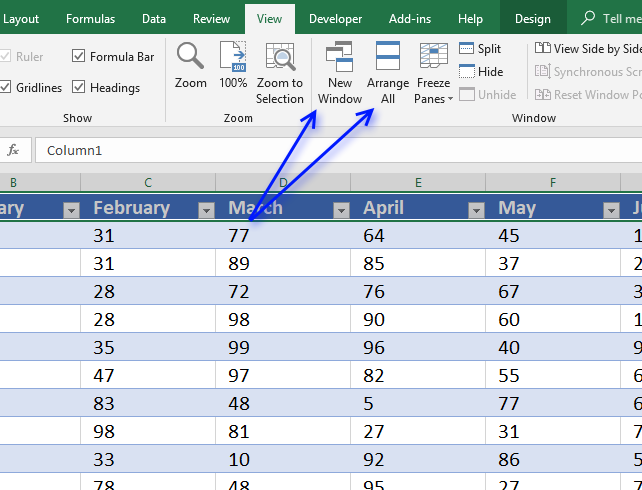
You can create a new window of the same workbook by pressing the "New Window" button on tab "View" on the ribbon.
The press with left mouse button on the "Arrange All" button to arrange windows. Select check box "Windows of active workbook" to only arrange the current workbook.
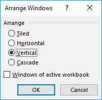
- Tiled is good for many different windows.
- Horizontal and Vertical is, in my opinion, best for two worksheets.
- Cascade lets you see all Excel window names in a nice layout.
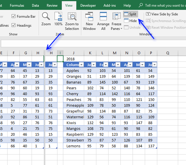
Use the Split button found on tab "View" on the ribbon to divide the same worksheet into two or more views.
This allows you to scroll each view independently letting you examine, for example, two different datasets, located on the same worksheet, simultaneously.
If you select a cell next to the column letters or row numbers and then press with left mouse button on the "Split" button Excel will divide the worksheet into two windows, see image above.
Any other cell selected will divide the view into four different windows.
Tip! Press and hold on a split line and then drag to change its location.
14.7. Create a chart
Insert a chart to create a better experience and enhancing the message you want to send.
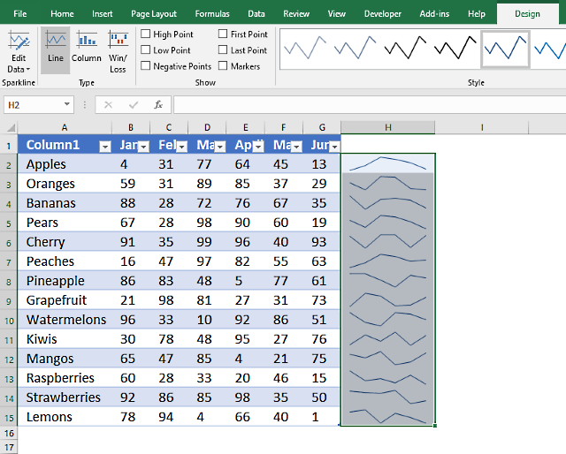
14.8. Use sparklines to visualize data
Sparklines is a new tool in Excel 2010, it visualizes data in a single cell in a simplistic form. No x and y-axis only the line.
- Select the cell range containing the data you want to use.
- Go to tab "Insert" on the ribbon.
- Press with left mouse button on "Sparklines" button.
- The data range should now be selected, you will only need to select the location of the spark lines.
- Press with left mouse button on OK button.
14.9. Highlight every other row
The following article explains how to highlight every other row using Conditional Formatting.
Recommended articles
Here is how to highlight every other row using conditional formatting. Conditional formatting formula: =ISEVEN(ROW())*OR($B3:$D3<>"") Alternative CF formula: =EVEN(ROW())=ROW() This […]
14.10. Highlight selected row

This article explains how to highlight the row or column based on the selected cell.
Recommended articles
Today I would like to share with you these small event handler procedures that make it easier for you to […]
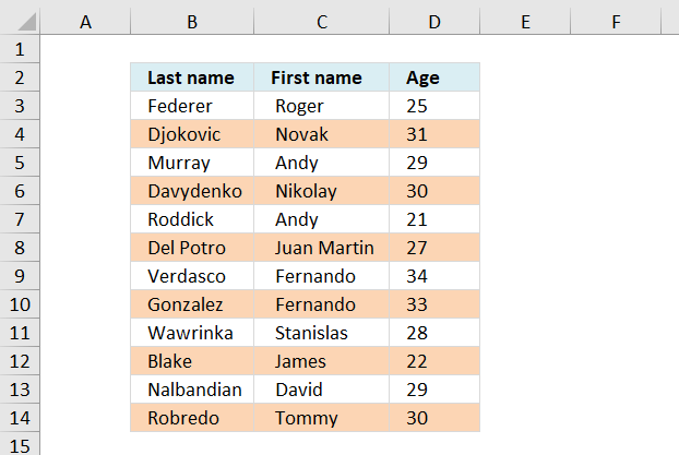
15. How to quickly select a cell range
Selecting cell ranges in Excel can sometimes be a real pain scrolling forever it seems. There is a quick and easy way to do it if you know the exact cell reference follow these simple steps.
- Type the cell reference in the name box.
- Press Enter.
- The cell range is now selected.
Excel references cells using a column letter and a row number called A1 reference style, for example, the first cell at top left has the address A1.
16. How to quickly select a named range or an Excel table
You can also use the technique described in section 1.1 above to select named ranges and Excel defined tables. Simply type the name of the named range or the name of the Excel defined Table to quickly move and select to that object.
The animated picture above demonstrates how to select an Excel defined Table using the name box.
17. Select a contiguous cell range
If you don't know the exact cell reference to a table or list simply press with left mouse button on a non-empty cell in the range you want to select and press CTRL + A.
This will select the cell range as long as it is a contiguous cell range, the above animated picture shows this technique.
18. How to name a cell range
The name box allows you to quickly name a cell or cell range, this is useful if you often use a cell value in a formula.
Revenue2017 is easier to remember than cell reference AB153.
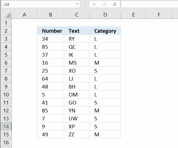
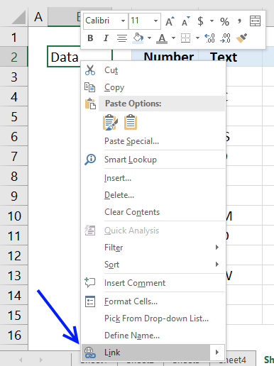
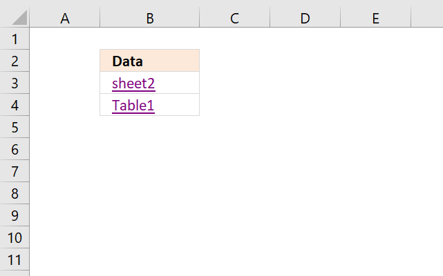
19. How to link to a specific cell range
Excel allows you to insert a hyperlink that points to a webpage, however, most people don't know that you can build a link that points to a cell range.
Here are the steps I made to build a hyperlink that selects cell range D3:F15:
- Type Data in cell B2 and then press Enter.
- Press with right mouse button on on cell B2 and select "Link"
- Press with mouse on "Place in This Document"
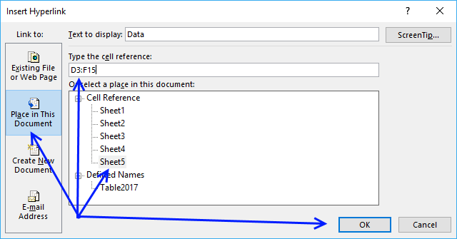
- Type D3:F15 in field "Type the cell reference:"
- Press with left mouse button on OK button
The following post explains how to build a cell link using a formula that lets you instantly select a cell range or an Excel defined Table.
The advantage with formulas is that you can make them dynamic meaning they are instantly refreshed and updated if a cell value changes.
Recommended articles
The image above shows two hyperlinks, the first hyperlink lets you select a data set automatically based on a dynamic […]
20. Different ways to delete a cell value

First, I want to show you how to delete a value in a cell. If you select the cell and then press the "Delete" key on the keyboard only the value or formula is deleted, not the cell formatting or the cell itself.
To delete the cell formatting as well you need to go to tab "Home" on the ribbon and press with left mouse button on "Clear" button. A pop-up menu shows up containing these actions:
- Clear All
- Clear Formats
- Clear Contents
- Clear comments and notes
- Clear Hyperlinks
- Remove hyperlinks
Press with mouse on "Clear All" to delete the value and the cell formatting.
The shortcut keys to clear all are Alt + H + E + A. "Clear All" will remove the values, formulas, cell formatting, comments, notes, and hyperlinks from the selected cell or cell range.
21. Delete a single cell

To delete a single cell entirely (with or without a value) press with right mouse button on on it to show a pop-up menu or context menu, press with left mouse button on "Delete...". A dialog box appears with the following options:
- Shift cells left - deletes the selected cell and move cells left to fill the deleted cell.
- Shift cells up - deletes the selected cell and move cells up to fill the deleted cell.
- Entire row - Deletes the entire row even if there are other non-empty cells on the same row. There is not even a warning, Excel deletes the entire row.
- Entire column - Deletes the entire column even if there are other non-empty cells in the same column. There is not even a warning, Excel deletes the entire column without a prompt.
You can use this method to delete all blank cells, see next section below.
22. Select and delete blank cells

- Select the cell range.
- Press function key F5 to open the following dialog box.
- Press with left mouse button on "Special..." button and the following dialog box appears.
- Select radio button "Blanks", see picture above.
- Press with left mouse button on "OK" button.

- Press with right mouse button on on any of the selected cells and press with left mouse button on "Delete..." on the pop-up menu.
- Press with left mouse button on "Shift cells up" on the dialog box.
- Press with left mouse button on OK button.

23. Select and delete cells matching a given condition

The image above shows a formula in column C that returns text string "Above" if the corresponding value in column B is above or equal to 50. If the number is below 50 then nothing is returned.
Formula in cell C3:
Excel is also able to select visible cells only, if we apply a simple filter to the table we can select the blanks and delete them. This allows you to filter cells based on any condition and then delete them.
- Go to tab "Data" on the ribbon.
- Press with left mouse button on "Filter" button or press shortcut keys CTRL + SHIFT + L. Arrows next to the header names appears.

- Press with mouse on the arrow next to the header name Formulas and a pop-up menu appears.

- Deselect checkbox next to "Above" to filter blanks.
- Press with left mouse button on OK button.

The row numbers and the arrow button shows that a filter is applied to the data, see image above. Select all blanks, in my example that would be cell C3, C4, C7, C9 and C10.
Press Function key F5 on your keyboard, press with left mouse button on "Special..." button.

Press with left mouse button on radio button "Visible cells only" and then press with left mouse button on OK button.

Press with left mouse button on "Delete row" on the pop-up menu, see image above. This will delete all rows containing a blank in column C.

Press with mouse on the button next to the header name "Formulas" and a pop-up menu shows up. Press with mouse on 'Clear Filter From "Formulas"', this will show whats left of data table.

24. Macro deletes formulas that return a blank
If you don't want to use the above technique or perhaps can't, the following macro deletes formulas evaluating to an empty text string:
'Name macro
Sub DeleteBlankRows()

'Iterate through selected cells
For i = Selection.Cells.Count To 1 Step -1

'Check if cell length is zero
   If Len(Selection.Cells(i)) = 0 Then

      'Delete cell
      Selection.Cells(i).Delete xlUp

   End If

'Next cell
Next i
End Sub
24.1 Where to put the VBA code?

The following steps shows how to add VBA code to your workbook. VBA stands for Visual Basic for Applications and it allows you to create custom-built programs or Excel Functions.
- Copy above VBA code.
- Press short cut keys Alt+ F11 to open the Visual Basic Editor (VB Editor).
- Press with left mouse button on "Insert" on the top menu, see image above.
- Press with left mouse button on "Module".
- Paste VBA code to code window.
- Exit VB Editor and return to Excel.
24.2 How to run the macro
- Select a cell range.
- Press Alt + F8 to open the macro dialog box.
- Select macro "DeleteBlankRows".
- Press with left mouse button on Run.
25. Macro deletes entire row if the formula returns blanks
This macro deletes the entire row if cell formula evaluates to an empty text string:
'Name macro
Sub DeleteBlankRows()

'Go through all selected cells
For i = Selection.Cells.Count To 1 Step -1

   'Check if cell length is zero
   If Len(Selection.Cells(i)) = 0 Then

      'Delete entire row
      Selection.Cells(i).EntireRow.Delete xlUp

   End if

Continue with next cell
Next i
End Sub
Blank cells category
More than 1300 Excel formulasExcel categories
127 Responses to “Cleaning Up Excel Worksheets: Eliminating Blank Cells, Rows, and Errors”
Leave a Reply
How to comment
How to add a formula to your comment
<code>Insert your formula here.</code>
Convert less than and larger than signs
Use html character entities instead of less than and larger than signs.
< becomes < and > becomes >
How to add VBA code to your comment
[vb 1="vbnet" language=","]
Put your VBA code here.
[/vb]
How to add a picture to your comment:
Upload picture to postimage.org or imgur
Paste image link to your comment.
I would like to use exactly this function, but I cannot get your example to work. Why do you have semicolons in the formula?
It has to do with regional settings. UK and US have colons, and we use semicolons. I will soon change all formulas to UK/US settings.
I do not know why but wordpress changes "" (double quotation marks) to
[...] G1:G16 is where I create the unique list. The downside is that there are blanks where a duplicate is found. See this article on how to remove blanks: Remove blank cells [...]
[...] Filed in Uncategorized on Mar.20, 2009. Email This article to a Friend In a previous article Remove blank cells, I presented a solution for removing blank cells. This only worked for cells containing text. In [...]
How can I use these formulas in case if cells are only virtually blank, i.e. "" values are retruned in particular cells by IF functions? Is there any way to remove such cells from the list?
Alex,
This formula removes cells that seem to be blank but contains a space character:
=INDEX($A$1:$A$8, SMALL(IF(TRIM($A$1:$A$8)="", "", ROW($A$1:$A$8)-MIN(ROW($A$1:$A$8))+1), ROW(1:1))) + CTRL + SHIFT + ENTER copied down as far as needed.
This is excellent. Thank you!
Can you think of any way to do this within a Named Range?
E.g., so I can define a range called "FilteredList" which only contained the cells with values, and then refer to that list elsewhere in the sheet?
thanks!
(sorry: I should have been clearer. I want to do it with a named range only -- without creating a hidden sheet containing the filtered list or anything like that.)
Greg,
I am using the same example as in this blog post and Excel 2007.
1. I copied this formula
=INDEX($A$1:$A$10,SMALL(IF(ISTEXT($A$1:$A$10), ROW($A$1:$A$10),""),ROW(1:10)))
2. I created a new named range (rng) in the "Name Manager" and pasted the formula into the "Refers to:" field.
3. Press OK button with left mouse button!
3. I then selected a new range (D1:D9) and typed in formula field: =rng + CTRL + SHIFT + ENTER
The result were a list without blanks. I have never tried this before but it seems to work.
How about:
1. CTRL+END
2. CTRL+SHIFT+HOME
Is this what you mean to do?
Jamieson,
Yes! Much better!
Thanks for commenting!
Hi! can you do this using the transpose function? so when you transpose a column to a row it removes the blanks in the process?
Thanks!
Instead of the column to a row, do a row to a column.
Arielle,
=INDEX($E$1:$K$1, 1, SMALL(IF(ISTEXT($E$1:$K$1), COLUMN($E$1:$K$1)-MIN(COLUMN($E$1:$K$1))+1, ""), ROW(A1))) + CTRL + SHIFT + ENTER. Copy cell and paste down as far as needed.
That is great thanks!! it works perfect!!! Now is it possible to do that exact formula to ignore cells that have the virtual blank ""?
not ignore i mean remove im sorry
Arielle,
=INDEX($E$1:$L$1, 1, SMALL(IF(LEN($E$1:$L$1), COLUMN($E$1:$L$1)-MIN(COLUMN($E$1:$L$1))+1, ""), ROW(A1))) + CTRL + SHIFT + ENTER. Copy cell and paste down as far as needed.
Oscar,
unfortunately that did not work :/. It did the same thing as the previous formula you gave me, which works great, but the new formula isn't removing the cells that have a space in it
Arielle,
Now I understand, try this formula:
=INDEX($E$1:$L$1, 1, SMALL(IF(LEN(TRIM($E$1:$L$1)), COLUMN($E$1:$L$1)-MIN(COLUMN($E$1:$L$1))+1, ""), ROW(A1))) + CTRL + SHIFT + ENTER. Copy cell and paste down as far as needed.
thanks that works great!!!!!
I have extracted a unique list from a list containing blanks ("LIST" is the named range), using this formula in Excel 2007:
=INDEX(LIST, SMALL(IF(TRIM(LIST)="", "", ROW(LIST)-MIN(ROW(LIST))+1), ROW(1:1)))
This works beautifully, except for one small thing. I need the unique list to display within a set number of rows, however the range "LIST" varies in size. I do not want #NUM! to display in the cells below the unique list. How can I make the cells below the unique list look blank, rather than displaying #NUM! ?
Laura,
=IFERROR(INDEX(LIST, SMALL(IF(TRIM(LIST)="", "", ROW(LIST)-MIN(ROW(LIST))+1), ROW(1:1))),"") + CTRL + SHIFT + ENTER. Copy cell and paste down as far as needed.
Oscar, I just changed your semicolon (near the end of the formula) to a comma, and it worked PERFECTLY. Thank you for your help!
For anybody else who is wondering: this actually doesn't select a non contiguous range like it says in the header.
Within the article the statement changes to "non contiguous list" which is correct (though i'm not sure if this term even exists in excel lingo).
To explain using the example table from the article:
Non contiguous range: A1:A5,A7:A12,A14:A18
Non contiguous list: A1:A18
After doing what is described in the article A1:A18 is selected and not the non contiguous range.
Johannes,
As far as I know, a cell range can be anything from:
One single cell
A column or row
Multiple columns and rows
If I remember it correctly, my intention was to describe how to select cell range containing blank cells or blank rows/columns quickly.
This is awesome!! I have been searching the internet looking for just this. One question though why does this not work?
=IF(SUM(IF(A1:A10"",1,0))>=ROW(),IF($V$4:$V43="space","",INDEX($V$4:$V43,SMALL(IF(TRIM($V$4:$V$43)="","",ROW($V$4:$V$43)-MIN(ROW($V$4:$V$43))+1),ROW(1:43)))),"")
Basically i took the formula that removes seemingly blank cells and tried to combine it will the one that removed the #NUM!?
The formula with out the beginning IF part works great.
Can this be done to remove the #NUM!? too?
Thank you!
Additional... i did make the initial IF statement have the array v4:v43 i just forgot to put that correct in the post. Thank you
Sam,
Read this: Delete blanks and errors in a list
Excel 2007:
IFERROR(value;value_if_error) Returns value_if_error if expression is an error and the value of the expression itself otherwise
Thanks for commenting!
I dont know why it is not working on me "+ CTRL + SHIFT + ENTER. Copy cell and paste down as far as needed." What I do is just drag the formula down up to the last cell I need. I am not sure if it is correct.
I really dont know what is wrong please help thanks
JOshua,
I am not sure what is wrong.
$B$3:$B$10 is the cell range. Adjust range to your sheet.
A1 (bolded) is a relative cell reference. This cell reference changes when you copy the formula.
Yes, you can also copy the formula by Press with left mouse button on and hold and drag the cell down to the last cell you need.
Wondering if you can help.
Easiest to put an example down:
CURRENT TRYING TO DO WOULD BE IDEAL
A B A B A B
Name 1 Data 1 Name 1 Data 1 Name 1 Data 1
Name 2 Name 3 Data 2 Name 4 Data 1
Name 3 Data 2 Name 4 Data 1
Name 4 Data 1 Name 6 Data 3
Name 5
Name 6 Data 3
Where the name stays matched up with the data item in the same row. I would think using hlookup or vlookup in some fashion might help but I can't wrap my brain around it. Any thoughts?
Well that doesn't look pretty how about this:
CURRENT TRYING TO DO WOULD BE IDEAL
--A--------B-----------A--------B-----------A--------B
Name 1...Data 1------Name 1...Data 1------Name 1...Data 1
Name 2...______------Name 3...Data 2------Name 4...Data 1
Name 3...Data 2------Name 4...Data 1
Name 4...Data 1------Name 6...Data 3
Name 5...______
Name 6...Data 3
Basically I'm looking to do the same thing the filter does but what I want to end up with is a single sheet that has 10 of these filterd lists above and next to each other.
Sorry - I found a work around using your current formulas above, glad I found it! Going to take some doing to set it up but it will be worth it.
Thanks!
Great to see a non-volatile solution to this problem.
If the apparently empty cell is "" returned by a formula then the "blanks" will not be removed,in fact as they are all read as different "blanks" and the list can/will remain unchanged.
This mod seems to handle this situation.
=INDEX($B$2:$B$200, SMALL(IF(($B$2:$B$200="")+ISERROR($B$2:$B$200), "", ROW($B$2:$B$200)-MIN(ROW($B$2:$B$200))+1), ROW(1:1)))
Wrap in IFERROR("formula","") for 2007 and above, or IF(ISERROR("formula"),"","formula") for 2003 and earlier.
Marcol,
Yes you are right. ISERROR($B$2:$B$200) removes formulas that return an error.
[...] how it can be done using formulas. One of them that explained how it can done can be found a https://www.get-digital-help.com/excel-remove-blank-cells/ modified the formula to do it for columns. Thennbsp;I setup the formulanbsp;such thatnbsp;he [...]
Oscar,
Thank you sooo much~!The formula removes cells that seem to be blank but contains a space character solve all my problems~!
Thank you SO MUCH for this!!!!!!!!!! I've been trying to write if statements for the last 2 days to try to filter out unneeded data. I just converted the garbage to blank cells then used your equation..... ITS Beautiful!!!!!!!
Thanks so much!!!
[...] available options and did not have blank spaces between them. I hunted on the internet and found an example, but it used functions that are not available in the Xcelsius-enabled list of Excel [...]
Hi Oscar,
I read your blog almost everyday. I found a lot of solution for interesting task here. I want to ask you for help. I tried to find solution for removing blank cells not in one column, but in range with few columns. Because the range is dynamic it possible to be from 1, 2, 3 or more columns.
I have a range similar like this:
A B C D E F
1 x x
2 x x
3 x
4
5 x
6
7
8 x x
The result must be:
1
2
3
5
8
Do you think that is possible without VBA?
One way might be to try this variation with the aid of a helper column.
Add two columns before Column A in your worksheet, or start your data table in Column C. Put as many as many headers as you need in Row 1 (These must be text strings for this example, dates as headers require a slightly different formula)
In B2
=IF(C2="","",COUNTIF(D2:INDEX(2:2,1,MATCH(REPT("z",255),$1:$1,1)),">"""))
Drag /Fill Down as required
In A2, this Array formula
=INDEX($C$2:$C$200, SMALL(IF(($C$2:$C$200="")+ISERROR($C$2:$C$200)+(--($B$2:$B$200=0)), "", ROW($C$2:$C$200)-MIN(ROW($C$2:$C$200))+1), ROW(1:1)))
Confirm with Ctrl+Shift+Enter, not just enter
Drag /Fill Down as required
Column B is a count of your "x" "flags", it could be hidden.
If your "flag" headers are serial dates change this
"REPT("z",255)" to "99^99" in B2.
Sorry, should have added this to the above post ...
Wrap (A2) in IFERROR("formula","") for 2007 and above, or IF(ISERROR("formula"),"","formula") for 2003 and earlier.
Hi Marcol,
With helper column is easy :) In fact with using helper formula the task is the same - "Remove empty cell ls in one column (helper)". I wonder if there is way to find non-blank lines from multi column table.
In fact yesterday I found way to do that, but the way is not so good in my opinion. I mean that if table is with a lot of columns it will be not possible to use the formula. I tried to made the formula unique - for 2, 3, 4 or more columns, but in the beginning it works for 2 or 3 columns, but for 4 failed to give results. I made some modifications and the formula start to work for 2, 3 or 4 columns... But the number of columns is still limitation - if I need to check more than 4 column table I need to integrate in formula more IFs (the same number as columns).
On Monday I will post the formula to see what I mean.
@ BatTodor
I'm not sure that I'm following you.
See if you can get this sample file from my skydrive.
https://skydrive.live.com/?cid=1760EAB0F9AE526F#!/view.aspx?cid=1760EAB0F9AE526F&resid=1760EAB0F9AE526F%21125
Add as many column headers as you want/need, then put "x" in any row in any column.
Hi Markol,
Thank you for solution! :)
I will try to find solution without helper column :)
BatTodor ,
I am not sure I understand.
What is x in your table?
Can you provide the formula you are working with?
Hi Oscar,
In general I want to know all rows which are not empty. "X" mean that (for example) number 1 is appeared in Column B and C. The task is became more complicated because I work with dynamic ranges and it could be one range to be with 1 or 2 or 3 or more columns. I wanted to create one formula for all cases – even the range grows to 10 or more columns. I modified your formula with integrated IFs, but for some strange reason formula failed to give results in some cases for 3 or 4 columns (for now the cases is with maximum 4 columns). After that I modified again formula and put one more IF – if there is 2 or more columns.
The final formula looks like this:
=INDEX(AllRanges;3+SMALL(IF(ISBLANK(INDEX(SelectedRange;;1)); IF(ISBLANK(INDEX(SelectedRange;;2));IF(COLUMNS(SelectedRange)>2;IF(ISBLANK(INDEX(SelectedRange;;3));IF(ISBLANK(INDEX(SelectedRange;;4));"";ROW(INDEX(SelectedRange;;4))-MIN(ROW(INDEX(SelectedRange;;4)))+1);ROW(INDEX(SelectedRange;;3))-MIN(ROW(INDEX(SelectedRange;;3)))+1);"");ROW(INDEX(SelectedRange;;2))-MIN(ROW(INDEX(SelectedRange;;2)))+1); ROW(INDEX(SelectedRange;;1))-MIN(ROW(INDEX(SelectedRange;;1)))+1); ROW(1:1));3)
I have 2 worksheet – in Worksheet1 is database and Worksheet2 is for calculations.
Where AllRanges is
=OFFSET(Worksheet1!$A$1;0;0;COUNTA(Worksheet1!$C:$C)+2;COUNTA(Worksheet1!$1:$1))
SelectedRange is
=OFFSET(Worksheet1!$A$1;3; Worksheet2!$G$2-1;COUNTA(Worksheet1!$C:$C)-1; Worksheet2!$F$2- Worksheet2!$G$2+1)
On Worksheet2 on cell C4 there is cell for choosing. From this choose SelectedRange is defined.
Again on Worksheet2 on cells F2 and G2 there are array formulas to calculate last and first columns for the range which was choosen
=MAX(IF(Worksheet1!3:3=$C$4;COLUMN(Worksheet1!3:3)))
=MIN(IF(Worksheet1!3:3=$C$4;COLUMN(Worksheet1!3:3)))
I hope that I was able to describe situation :)
Ups, I saw that the formula is not clear for reading :(
=INDEX(AllRanges;3+SMALL(IF(ISBLANK(INDEX(SelectedRange;;1)); IF(ISBLANK(INDEX(SelectedRange;;2));IF(COLUMNS(SelectedRange)>2;
IF(ISBLANK(INDEX(SelectedRange;;3));IF(ISBLANK(INDEX(SelectedRange;;4));"";
ROW(INDEX(SelectedRange;;4))-MIN(ROW(INDEX(SelectedRange;;4)))+1);
ROW(INDEX(SelectedRange;;3))-MIN(ROW(INDEX(SelectedRange;;3)))+1);"");
ROW(INDEX(SelectedRange;;2))-MIN(ROW(INDEX(SelectedRange;;2)))+1);
ROW(INDEX(SelectedRange;;1))-MIN(ROW(INDEX(SelectedRange;;1)))+1); ROW(1:1));3)
hi, thanx 4 your valuable formulas
i have a query, if u help i will be very thankful....
i have a workbook which is having 2 worksheet
i sheet1 i have a data range C1:H100
i just want a formula with this criteria
if i type "OK" in any column rang from J1:J100
the same row which cell contains "OK" match with other 6 rows range
and return the data in sheet2 with ignoring the blank calls
the data should be return in first row
and it should follow the same criteria when in put "OK" in any other column eg:
Sheet1 sheet2
C D E F G H J C D E F G
1 4 5 2 11 "OK" 1 2 4 5 11
please help me for this
i will be very thankful to u all
This is an amazing piece of code.
8-)
BatTodor,
I modified the formula in this post:
Unique distinct values from multiple columns using array formula
This formula works with blanks.
SUNNY,
the same row which cell contains "OK" match with other 6 rows range
Can you explain in greater detail?
Matt Villion,
thanks!
Hi Oscar,
Thank you very much for your reply, but the formula which you send me isn't give result in my case...
It's my mistake - sorry for my poor English :( In my example the digits on first columns are the rows numbers, not entered digits.
The task looks like this "Remove blank rows from multi-column array". I want to know which rows contains data (I marked with "X") on one or more cells (columns).
Hi Oscar,
thanx for giving me ur valuable time
after one day if mind exercise i came to conclusion and this formula works for me but it slowdown my excel file processing.
if possible can you help for the above mention problem
{=IFERROR(IF(V4="OK",INDEX(K4:O4, SMALL(IF(ISBLANK(K4:O4), "", COLUMN(K4:O4)-MIN(COLUMN(K4:O4))+1), COLUMN(A3))), ""),"")}
thanx again
BatTodor,
Check out this formula:
https://www.get-digital-help.com/wp-content/uploads/2007/09/Remove-blanks-from-a-cell-range.xlsx
Unfortunately it is a complicated formula, I wish I could make it smaller.
hi oscar,
is there any formula that can replace a rang of cells value into text
eg:
A B C D E W
1 3 4 6 8
2 4 5 7 9 OK
1 2 6 8 3
now i want to replace the value 1 with (oscar)
is it possible with formula.
one more question is that:
is that any formula which can lookup the cell rang W2:W321 & if any cell contains "OK" then it lookup the cell rang in the same row i.e. A:E
and then count the value just like in example.
thanks in advance
Hi Oscar,
THANK YOU VERY MUCH for solution! :) In fact for my current task which I try to solve is enough to know the numbers of non-empty rows and this part of your formula gives needed information =SMALL(IF(FREQUENCY(IF(List"";MATCH(ROW(List);ROW(List));"");MATCH(ROW(List);ROW(List)))>0;MATCH(ROW(List);ROW(List));"");ROW(A2)). In any way it will be big challenge for me to understand the formula :)
In general for me is interesting to know the way for creating array formulas – how to trace results, how to choose when use array formula "row-by-row" instead "for-all-area" (I'm not sure that I wrote it right), etc. I read your blog often, but the logic for array formulas is very big challenge for me.
In the past it was like a magic – now I see that you started to explain very detailed the reason of using parts of formulas :) And now it comes to cleared the picture, but still is hard for me to create my own array formulas.
In any way again want to thank you Oscar!
SUNNY,
You can´t replace a value in another cell using a formula. A formula can only return a value in the cell it is entered.
and then count the value
Can you explain in greater detail?
The best one:
G14:G19 is the array with blanks and non-blanks. Put it in the first target cell in the column of results. With cursor in formula bar, press Control+Shift+Enter. Now drag it along the entire range.
johnson,
thanks for sharing!
Thank you Oscar,
Your approach is great and works fine. I used several hours to find such a solution.
Keep on sharing the knowledge.
Idrissa
Idrissa,
thanks for commenting!
Hello,
I am having the same issue as above with a little twist. Have 4 active wsorksheets in a workbook. Each worksheet has formulas that pull data from the another worksheet. What I need to do is combine one formula with another formula that will pull over the data as well as delete any blank rows. The formula that I have which is pulling over data is: Column A: =IF(Modifications!C4="Open / Active","A",IF(Modifications!C4="Completed","D","")). Modifications being one of the active worksheets. Column B: =IF(Modifications!A4="","",Modifications!A4). Currently, its pulling the data correctly but there are blank rows, I need those deleted and can't figure out how to combine the formulas. Please help!!
BTW, I am comparing a current worklist with a new worklist that will let me know what I need to upload as an Add or Delete.
Lisa S,
See attached file:
Remove-blank-rows.xlsx
Thank you for the great work Oscar!
I found your remove blank rows array formula to be especially helpful. Is it also possible to add another condition onto that? For instance, using your example, would you be able to remove blanks and list only the rows of people over the age of 30?
Thank you for your help!
Yen,
Thanks!
Is it also possible to add another condition onto that? For instance, using your example, would you be able to remove blanks and list only the rows of people over the age of 30?
Yes, it is possible!
Array formula in cell E2:
Thank you Oscar! This formula is exactly what I've been searching for. I just wanted to thank you for the excellent resource you are providing!
Thank you for commenting!
Oscar, thank you so much! I had a chance to test your solution and it works beautifully.
I had no idea about the option to use * in an IF function to accommodate multiple conditions. This will definitely make my life a bit easier :)
I'm going crazy trying to figure this one out...
Sorry to bring you back to the olddays of yore, but I'm still using Excel 2003... (don't laugh-it was free!)
I'm, as you can guess, trying to remove blank lines. I haven'ttried allof the formulas on the ->https://www.get-digital-help.com/excel-remove-blank-cells/ =INDEX($B$3:$B$10, SMALL(IF(ISBLANK($B$3:$B$10), "", ROW($B$3:$B$10)-MIN(ROW($B$3:$B$10))+1), ROW(A1))) =IFERROR(INDEX($B$3:$B$10, SMALL(IF(ISBLANK($B$3:$B$10), "", ROW($B$3:$B$10)-MIN(ROW($B$3:$B$10))+1), ROW(A1))), "") <-)
There are three problems with these formula (actually, with me):
(1) I don't know how to modify these formulas to my range (A59 to I129)
(2) This formula creates a #NUM error in the resulting array if the cell in the source array is blank. I don't know how to modify the formula to show blank cells instead of an error. (Yes, I want to show blank cells, not #NUM error indicators.)
(3) I don't know how to modify the second formula to Excel 2003.
Can someone help?
Thanks
hendis
hendis,
This formula should work in excel 2003:
=IF(ISERROR(INDEX($B$2:$C$9, SMALL(IF(FREQUENCY(IF($B$2:$C$9<>"", MATCH(ROW($B$2:$C$9), ROW($B$2:$C$9)), ""), MATCH(ROW($B$2:$C$9), ROW($B$2:$C$9)))>0, MATCH(ROW($B$2:$C$9), ROW($B$2:$C$9)), ""), ROW(A1)), COLUMN(A1))), "", INDEX($B$2:$C$9, SMALL(IF(FREQUENCY(IF($B$2:$C$9<>"", MATCH(ROW($B$2:$C$9), ROW($B$2:$C$9)), ""), MATCH(ROW($B$2:$C$9), ROW($B$2:$C$9)))>0, MATCH(ROW($B$2:$C$9), ROW($B$2:$C$9)), ""), ROW(A1)), COLUMN(A1)))
Using your cell references:
=IF(ISERROR(INDEX($A$59:$I$129, SMALL(IF(FREQUENCY(IF($A$59:$I$129<>"", MATCH(ROW($A$59:$I$129), ROW($A$59:$I$129)), ""), MATCH(ROW($A$59:$I$129), ROW($A$59:$I$129)))>0, MATCH(ROW($A$59:$I$129), ROW($A$59:$I$129)), ""), ROW(A1)), COLUMN(A1))), "", INDEX($A$59:$I$129, SMALL(IF(FREQUENCY(IF($A$59:$I$129<>"", MATCH(ROW($A$59:$I$129), ROW($A$59:$I$129)), ""), MATCH(ROW($A$59:$I$129), ROW($A$59:$I$129)))>0, MATCH(ROW($A$59:$I$129), ROW($A$59:$I$129)), ""), ROW(A1)), COLUMN(A1)))
See attached file:
Remove-blank-rows-from-a-cell-range-formula-excel2003.xls
Oscar, thank you for the comment, formula and file.
(One look at the formula you put together tells me that there is no way in the world that I would - or could - have figured this thing out.)
Unfortunately, when I copy and paste your formula into my spreadsheet, I get an error. When I open the Excel 2003 file you included, the spreadsheet shows a VALUE error, but nothing else -- no formula, no text, no nothing.
What am I doing wrong?
hendis
hendis,
My formula uses more levels of nesting than are allowed.
Try this formula:
See attached file:
Remove-blank-rows-from-a-cell-range-formula-excel2003_2.xls
Hi Oscar,
I am trying to use your array formula
=INDEX($C3:$AO3,SMALL(IF(ISBLANK($C3:$AO3),"",COLUMN($C3:$AO3)-MIN(COLUMN($C3:$AO3))+1),COLUMN(A1)))
on values collected using the CONCATENATE function, some of which are zeros. Most of the cells in my row arrays don't return a value but contain the concatenate formula and therefore aren't removed by the above.
Can ISBLANK or another part of the formula be easily adapted to remove cells that don't return a value (showing those that return a zero) but do contain a formula.
Look forward to hearing from you,
Matt
Matt,
Try this array formula:
=INDEX($C3:$AO3, SMALL(IF(ISERROR($C3:$AO3), "", IF($C3:$AO3="", "", MATCH(COLUMN($C3:$AO3), COLUMN($C3:$AO3)))), COLUMN(A1)))
That works perfectly, really appreciate the help!
Hi Oscar,
I've successfully implemented one of your fabulous formulas, but am now stuck on a variation. I am trying to pull names (found in 'Pre-Separation Sign-Up'!C25:C225) of people who have completed at least one section of a course, but not all of it. Incomplete sections are marked "Incomplete" in rows W:BT. Complete sections are left blank.
I think I need to use COUNTBLANK across a dynamic range as part of the selection criteria. I've made a failed attempt inside the second IF statement below. What I want is to count the number of blanks (both real and formula produced) from W to BT (a subset of the larger A:BT range being used in the rest of the formula). If any of these are not blank, I want to import the data from that row. I know the rest of the formula works well, but I just can't quite get the syntax for the COUNTBLANK condition to cooperate.
=IFERROR(
INDEX('Pre-Separation Sign-Up'!$A$25:$BT$225&"",
SMALL(
IF(
FREQUENCY(
IF(('Pre-Separation Sign-Up'!$A$25:$BT$225"")*(COUNTBLANK('Pre-Separation Sign-Up'!$W$25:INDEX('Pre-Separation Sign-Up'!$W$25:$BT$225, MATCH(2,1/'Pre-Separation Sign-Up'!$W$25:$BT$225"")))0,
MATCH(
ROW('Pre-Separation Sign-Up'!$A$25:$BT$225),
ROW('Pre-Separation Sign-Up'!$A$25:$BT$225)), ""),
ROW('Pre-Separation Sign-Up'!$C1)),
COLUMN('Pre-Separation Sign-Up'!$C1)),
"")
Thank you in advance for your help!
-Katie
Oops, here's the bit I'm working on:
(COUNTBLANK('Pre-Separation Sign-Up'!$W$25:INDEX('Pre-Separation Sign-Up'!$W$25:$BT$225, MATCH(2,1/('Pre-Separation Sign-Up'!$W$25:$BT$225""))))<50)
Not quite sure what happened, but my first copy/paste just didn't come through correctly at all! Sorry for the multiple messages!
=IFERROR(
INDEX('Pre-Separation Sign-Up'!$A$25:$BT$225&"",
SMALL(
IF(
FREQUENCY(
IF(('Pre-Separation Sign-Up'!$A$25:$BT$225"")*(COUNTBLANK('Pre-Separation Sign-Up'!$W$25:INDEX('Pre-Separation Sign-Up'!$W$25:$BT$225, MATCH(2,1/('Pre-Separation Sign-Up'!$W$25:$BT$225""))))0,
MATCH(
ROW('Pre-Separation Sign-Up'!$A$25:$BT$225),
ROW('Pre-Separation Sign-Up'!$A$25:$BT$225)), ""),
ROW('Pre-Separation Sign-Up'!$C1)),
COLUMN('Pre-Separation Sign-Up'!$C1)),
"")
Katie G,
See attached file:
Katie-G.xlsx
Array formula in C11:
My Excel hero! Thank you! This worked beautifully!
Ok, so I'm having trouble developing an inventory spreadsheet using Microsoft Excel 2013. I have all of the inventory scanned in, but i am trying to set up a system that will delete a serial number from sheet 1 (warehouse inventory) when i scan the same serial number on subsequent sheets (2,3,4,5,6etc..) no matter what cell the serial number is in. Sheet 1 is the warehouse inventory and all of the others are inventory on different installation technician's trucks and I need to be able to assign them equipment with ease,as well as have the remaining blank cells in sheet1 be deleted automatically....I can't figure it out!!! Time to turn to smarter people PLEASE help!
I am trying to use the formula =IF(ISERROR(INDEX($X$13:$FN$13, MATCH(0, IF(ISBLANK($X$13:$FN$13), 1, COUNTIF($K$5:K8, $X$13:$FN$13)), 0))),"",INDEX($X$13:$FN$13, MATCH(0, IF(ISBLANK($X$13:$FN$13), 1, COUNTIF($K$5:K8, $X$13:$FN$13)), 0))) but I want to allow repeatition please help
Excellent, thank you! Took quite a few google searches to come across this. VERY simple and helpful!
Just two steps - Ctrl Space Bar, Ctrl shift up
I have been trying to find a formula to remove "blank" cells from list A and put then into a consolidated list B. The contents of list A is text and comes from a formula. the consolidated list B works some of the time, but when I change 1 of the inputs that generates list A list B doesn't work.
List A's formula is:
=INDEX($K$5:$P$250,-INT(-ROWS(Z$6:Z6)/$K$1),MOD(ROWS(Z$6:Z6)-1,$K$1)+1) where K5-P250 are the columns of the matrix of text. The matrix can vary in width from 4-6, which II manually input in cell K1 to = the number of columns in the matrix and the consolidated list starts in cell Z6. All works until I use a 4 column matrix and update cell K1 to a 4 or smaller number..
In Z6 I have tried:
=IFERROR(INDEX(Z$6:Z$1000,SMALL(IF($Z$6:$Z$1000"",ROW($Z$6:$Z$1000)-ROW($Z$6)+1),ROWS(AI$6:AI205))),"") Control+Shift+Enter again works great until I update K1 to a 4,3, or a 2 and all of Oscar's variations haven't helped.either.
Thanks for the help in advance.
Doug
Hi Oscar,
Just wanted to thank you for the absolutely incredible stuff you have posted here. At least three times, I have been able to apply your formulas to a project and make it awesome. Just fantastic.
K.
KW,
thank you for your kind words!
[…] For Excel for Windows, there’s an option to search a sheet for errors and go straight to them, under the “Find and select” icon in the ribbon. […]
In your article "How to extract a unique distinct list from a column in excel" (https://www.get-digital-help.com/how-to-extract-a-unique-list-and-the-duplicates-in-excel-from-one-column/) the formula (if you continue to copy it down past the last entry), will leave a "0" in the first cell after (i.e. b17) your last entry (i.e. Almagro, Nicolas in cell B16). Using the "IFERROR" function doesn't solve it (it does for the ensuing cells). Neither, that I can tell, do any of the options on this page. How would you change the formula [=IFERROR(INDEX(List,MATCH(0,COUNTIF($B$1:B1,List),0)),"")] to get rid of the "0" that will appear in cell B17.
Aaron,
I don´t get a "0". See this picture:
I'm using Excel 2013 in case that matters. See picture below. I get a "0" and then the "#N/A" after that. When I add IFERROR the "#N/A" becomes blank, but the "0" still exists.
https://s17.postimg.org/5flnfck8v/Page_1_Index_Example.jpg
Aaron,
How would you change the formula [=IFERROR(INDEX(List,MATCH(0,COUNTIF($B$1:B1,List),0)),"")] to get rid of the "0" that will appear in cell B17?
The named range List is larger than necessary. for example A2:A21 or your range contains a blank cell.
Yes, the list is larger than necessary on purpose. You should, theoretically, be able to autofill data using Index and Vlookup. Having a list larger than necessary allows room to accomodate users with different amounts of data. I ended up eliminating the "0" issue using an IF statement. I was just thinking there was another way. I'm using Excel 2013...maybe that is contributing to it... In any event, my fix worked even if it wasn't elegant. I will upload the file I did so you can see what I was doing and what I did to fix it (you don't need to do anything with it, it's just for your reference if your interested). I appreciate your help. Have a good one.
I am trying to make a workbook with two sheets. One sheet will have data including the prices of various items. Second sheet will have formatted invoice which will only receive selected data from the Sheet one. This selection in sheet one will be done by type Y or N in the end of every record. Those with N should NOT be in the invoice sheet and all with Y should be in invoice sheet without any blank records in it.
I have tried a lot your formula but it doesnt work. Struggling a lot to break it in small segments to work. Can you help me in this regard.
Also when I try =IF(LIST"",1,2) it results #Value!
Riz,
My email is [email protected]. If you want, I can send you a file I did that mirrors what you want to do close enough that you should be able to work out a solution for your situation.
Aaron
aaronb123...outlook.com. Fill in the @ at the ...
I have sent you an email Aaron.
I would like to use your
=INDEX($B$3:$B$10, SMALL(IF(ISBLANK($B$3:$B$10), "", ROW($B$3:$B$10)-MIN(ROW($B$3:$B$10))+1), ROW(A1)))
formula against an "Excel Table" (ie using Table Nomenclature), in such a way, that as the table grows in number of rows, the resulting array adjusts accordingly.
Can you advise?
Many thanks for your contribution and suppport.
Kind regards.
DMurray3,
see attached file:
DMurray3.xlsx
Many thanks Oscar... Your recommendation works like a charm...
Kind regards.
Oscar,
I am working with this formula to copy a long list of inventory from one tab to another. I want all the blanks to be skipped. This list will be updated 2-3 times a week. I am looking to only do this formula once and as inventory changes in the other tab, this "Master" list can change as well. Any help or solution?
Thank you.
[…] Excel: Remove blank cells | Get Digital Help – Microsoft … – Problem: Remove blank cells from a list of values? How to create a list with non empty cells? I want to create a new list without blanks. Answer: In this… […]
Tried a few different help forums trying to remove blank lines in a table and the formulas at the top work perfectly for me so thank you. I was just wondering if there's a way to return a different column of data?
i.e. when checking column A for blanks, I want to it return B3 even though it's blank just because A3 has data.
[…] Excel: Remove blank cells […]
hi all
anyone who can give advise of what to do when my file stops responding? i noticed it starts to not respond if i place the formula being discussed here. i have a very large file, about 1000 to 5000 KB. formula worked when tried in the first cell, but the file starts to not respond when i drag the formula down the other cells in a column..
Hi Oscar,
When I tried to copy your example for the Array Formula in cell D3, my new list just repeats "SM" all the way down the list, from D3 to D10. I can't figure out why this is the case. Can you help?
Never mind! I figured it out. If I do an array formula, ROW(A1) doesn't seem to iterate as we read down column B. But that does work if I just drag the formula down to fill the destination column; the iterating ROW(A1) works to select the k-th smallest value from the array.
However, for an array formula, I replaced ROW(A1) with ROW(A:A) so it iterates as we read down the column.
I'm pretty positive I'm not explaining myself very clearly... :-) but it makes sense to me! Thanks!
Excellent, thank you!
we can use conditional formatting too !!
Hi Oscar,
I am trying to delete blank cells but by shifting the cells left in the row. I don't want to delete the blank cells up as all my data is in rows. Do you a formula that can work? Let me know Thanks,
Thanks a lot Oscar. It helped me. its working awesome.
Hi,
I just can`t seem to get the formula working. I`m following the instructions, but the formula doesn`t remove empty cells. It merely Mirrors the table With alle empty cells. So now i have two tables With empty cells.
Can`t figure out what i`m doing wrong. I`m sure it`s something small and rediculous and i`m going insane trying to figure this out.
Here is my Version of Your formula:
=INDEX($D6$:$D$93; SMALL(IF(ISBLANK($D6$:$D$93); ""; ROW($D6$:$D$93)-MIN(ROW($D6$:$D$93))+1); ROW(A1)))
My blank cells contain the following formula
=IFERROR(IF(enrolled!F5="x";enrolled!C5;"");"")
I need those cells counted as blank and removed to get a proper list of enrolled pupils
Hi. do you have a tutorial on how to remove duplicates?
Elsie Serrano,
Sure, read this:
https://www.get-digital-help.com/how-to-extract-a-unique-list-and-the-duplicates-in-excel-from-one-column/
If I do an array formula, ROW(A1) doesn't seem to iterate as we read down column B. But that does work if I just drag the formula down to fill the destination column; the iterating ROW(A1) works to select the k-th smallest value from the array.
THis was very handy as teh latest version of Office 365 Win 10 has an Error Check (under Formulas tab) but it was not finding several errors. This method most most of them. They were hidden in merged cells where the left cell was find but the 3 to the right were not. THe last errors neither found were in tables where the #ref was not visible due to formatting.
Thank you so much. I was starting to go crazy.
Hello,
I am trying to remove blank rows from a list that I have in excel.
the list has 200 rows and 7 columns. Part of list ex. shown below:
Orriginal List:
8 8 8 8 8 8 8
5 2
3 5
3
2 3 1
What I want it to look like:
8 8 8 8 8 8 8
5 2
3 5
3
2 3 1
I tried using the formula you posted:
{=IFERROR(INDEX(List,SMALL(IF(FREQUENCY(IF(List"",MATCH(ROW(List),ROW(List)),""),MATCH(ROW(List),ROW(List)))>0,MATCH(ROW(List),ROW(List)),""),ROW(B1)),COLUMN(B1)),"")}
but it isnt working... Even when I take your excel example and paste it on my sheet it doesn't work...
Any suggestions?
Now I understand, try this formula:
=INDEX($E$1:$L$1, 1, SMALL(IF(LEN(TRIM($E$1:$L$1)), COLUMN($E$1:$L$1)-MIN(COLUMN($E$1:$L$1))+1, ""), ROW(A1))) + CTRL + SHIFT + ENTER. Copy cell and paste down as far as needed.
Thank you! This is my favorite excel formula so far.
Hi , I'm having trouble getting your formula to work properly in my sheet. Your formula works fine in your sheet but when I copy it into mine I cannot get **** excel to copy it while incrementing the row1:1 portion of the formula. I can copy the first cell identically into all cells in the column but that is no good. If I try to edit it I just get an error telling me I can't edit an array fomula. If I try to use "fill down" then the first cell works fine but all the others in the column return NUM or VAL errors! How the flip do I get **** excel to copy the formula down a column while incrementing the ROW1:1 to ROW2:2 etc?
This is driving me nuts!
Running windoze 10 home with whichever version of excel that shipped with.
Your formula does pretty much exactly what I need which is great- if I can just get it to increment those row numbers!
Help gratefully received!