Advanced Techniques for Conditional Formatting
Table of contents
- How to change cell formatting using a Drop Down list
- Highlight cells based on coordinates
- Highlight every other row
- Highlight opposite numbers
- Dynamic conditional formatting
- Highlight closest number
- Highlight cells based on numerical ranges
- How to highlight row of selected cell automatically using event macro - VBA?
- Highlight column of selected cell - VBA
- Highlight row and column of selected cell - VBA
- Highlight rows and columns of multiple selected cells - VBA
- Apply borders to row of the selected cell - VBA
- Get Excel macro-enabled *.xlsm file
1. How to change cell formatting using a Drop Down list

This article demonstrates how to apply different cell formatting to a cell range based on a Drop Down list, column B contains an Excel Table with numerical values.
The Drop down list in cell D3 lets you choose between five different types of cell formatting, they are:
- No formatting (General)
- % (percentage)
- Numbers formatted as time
- Highlight numbers below average
- Highlight numbers above average
You can, of course, pick whatever cell formatting you want and how many or few as you want. I chose those for demonstrational purposes.

The animated image above shows me selecting different formattings and column B instantly changes based on what I selected. This technique can be useful if you are building a Dashboard.
Here is how I did it.
Create an Excel Table

This step is optional, however, I highly recommend it if you know you will be adding more values later on.
An Excel Table applies Conditional Formatting to new values automatically, this makes it really useful because there is no need to extend CF formatting or change CF formulas when new values are added.
- Select all cells in your data set.
- Go to tab "Insert" on the ribbon.
- Press with left mouse button on "Table" button, a dialog box appears.
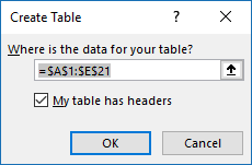
- Press with left mouse button on OK button.
You data set has now a different cell formatting applied, this is done every time data is converted to an Excel Table. You can change this if you like.
- Press with left mouse button on any cell in your Excel Table.
- Go to tab "Table Design" on the ribbon.
- Here you have plenty of Table Styles to choose from.
Create a Drop Down list

A Drop Down list lets you control what the user enters in a worksheet, press with left mouse button on the black arrow next to the cell to expand the list.
The list shows valid values the user can select, simply press with left mouse button on a value with the mouse or use up/down arrow keys.
- Select cell D3.
- Go to tab "Data" on the ribbon.
- Press with left mouse button on "Data Validation" button on the ribbon and a dialog box appears.
- Go to tab "Settings" on the dialog box. See image below.

- Select List
- Type: No formatting, %, Time, Above Average, Below Average
- Press with left mouse button on OK button to close the dialog box.
Apply Conditional formatting

Conditional Formatting allows you to format a cell or cell range based on a condition, in this case, the condition is given in cell D3 where we have a Drop Down list located.
We need to create five different CF formulas, each one applying different cell formatting to a column in the Excel Table.
For example, the image above shows that the selected value in the Drop Down list is "Above Average", the corresponding Conditional Formatting formula is activated and highlights values in Excel Table if a number is above the average of all numbers in the "Values" column.
Follow these steps to apply Conditional Formatting to column Values in the Excel Table.
- Select all values in column "Values".
- Go to tab "Home" on the ribbon.
- Press with left mouse button on the "Conditional Formatting" button and a menu appears.
- Press with left mouse button on "New Rule...".

- Copy this formula:
=($D$3="Above Average")*(INDIRECT("Table1[@Values]")>AVERAGE(INDIRECT("Table1[Values]")))
and paste to "Format values where this is true:" - Press with left mouse button on "Format..." button and pick a color. Cells that meet the requirement (return TRUE) in the above formula will be highlighted with this color.
- Press with left mouse button on OK button.
- Press with left mouse button on OK button once again to close the Conditional Formatting dialog box.
- Repeat step 1 to 8 with the remaining cell formattings.
Here are the formulas and formatting:
% formula
The formula checks if the value in cell D3 is %. If true the following formatting is applied:

Time formula
The formula checks if the value in cell D3 is Time. If true the following formatting is applied:

Above Average
In this formula, cell D3 is "Above Average" AND checks if each value is above the average of the table values. If TRUE the cell is highlighted.

Below Average

2. Highlight cells based on coordinates
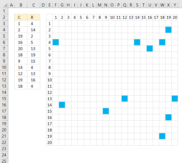
The picture above shows Conditional Formatting highlighting cells in cell range F3:Y22 based on row and column values in column B and C.
Conditional Formatting formula applied to cell range F3:Y22:
The first coordinate in cell range B3:C3 is column 1 and row 4, the conditional formatting formula highlights cell F6 because it is column 1 determined by the value in F2 and row 4 based on value in E6.
Explaining Conditional Formatting formula in cell F3
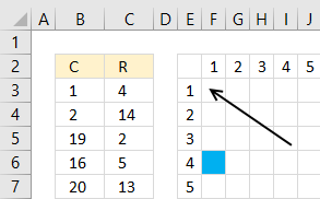
The COUNTIFS function counts the number of records in B3:C13 that match both the column (F$2) and row ($E3) value.
F$2 is 1 and $E3 is 1, no record in B3:C13 matches so cell F3 is not highlighted.
F$2 is locked to row 2 and $E3 is locked to column E so the cell references changes to F$2 and $E4 in next cell below. The dollar sign $ determines if a cell reference is absolute (locked) or relative.
How to apply conditional formatting formula to a cell range
- Select cell range F3:Y22.
- Go to tab "Home" on the ribbon.
- Press with mouse on the "Conditional Formatting" button.
- Press with mouse on "New Rule..."
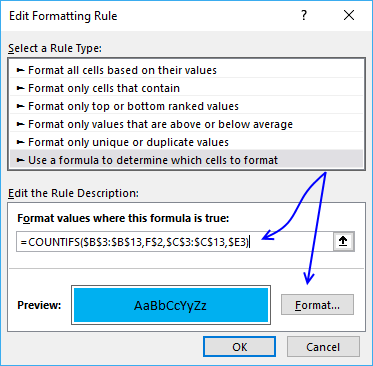
- Type the formula and then press with left mouse button on "Format..." button
- Press with mouse on tab "Fill"
- Pick a color
- Press with left mouse button on OK
- Press with left mouse button on OK button
Get Excel *.xlsx file
Highlight cells based on coordinates.xlsx
3. Highlight every other row
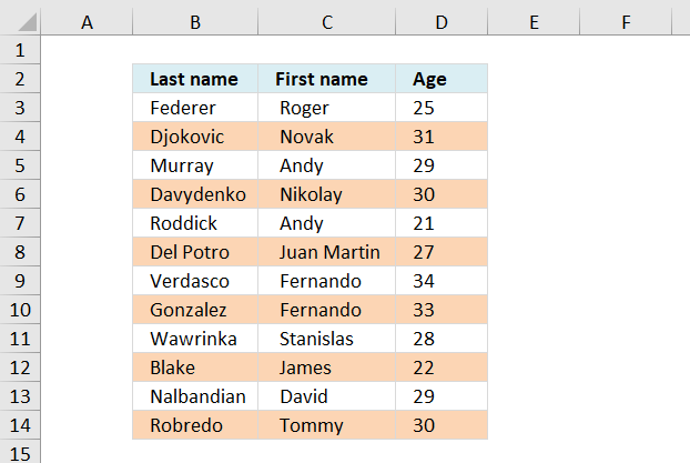
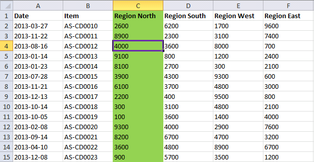
Here is how to highlight every other row using conditional formatting.
Conditional formatting formula:
Alternative CF formula:
This formula colors every second row if any cell in the row is populated. If you know you will add more records later to the list, select and conditional format a range larger than the list. Empty rows won´t be formatted.
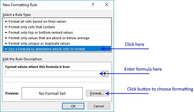
How to apply the conditional formatting formula in excel 2007:
- Select the range, example cell range A:C
- Press with left mouse button on "Home" tab on the ribbon
- Press with left mouse button on "Conditional formatting"
- Press with left mouse button on "New rule..."
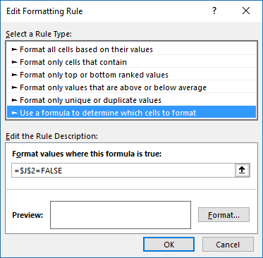
- Press with left mouse button on "Use a formula to determine which cells to format"
- Press with left mouse button on "Format values where this formula is true" window.
- Type =ISEVEN(ROW())*OR($B3:$D3<>"")
- Press with left mouse button on Format button
- Press with left mouse button on "Fill" tab
- Select a color
- Press with left mouse button on OK!
- Press with left mouse button on OK!
Explaining the contional formatting formula in cell A2
=ISEVEN(ROW())*OR($A2:$C2<>"")
Step 1 - Check if row number is even
ISEVEN(ROW())*OR($A2:$C2<>"") returns TRUE in cell A2.
Step 2 - Check if any of the cells in row are not empty
=ISEVEN(ROW())*OR($A2:$C2<>"") returns TRUE
Step 3 - Multiply functions (AND logic)
Both functions need to return TRUE in order to return TRUE
ISEVEN(ROW())*OR($A2:$C2<>"") returns TRUE. Row 2 is conditional formatted.
Get excel sample file for this tutorial
color-every-second-row-using-dynamic-conditional-formatting.xls
(Excel 97-2003 Workbook *.xls)
4. Highlight opposite numbers
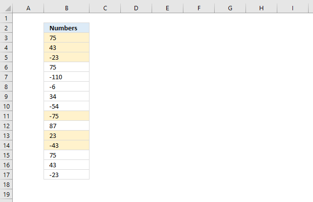
Pamela asks:
Ex. 1 with -1, 5000 with -5000, 75 with -75, etc.
Once I find those pairs, WITHOUT REPEATING
Ex. 75,-75,75, just the first TWO should get marked, and leave the last 75 alone.
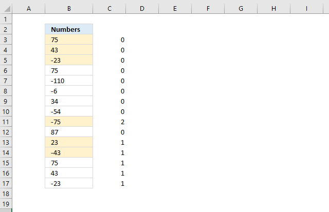
Conditional formatting formula applied to cell range B3:B17:
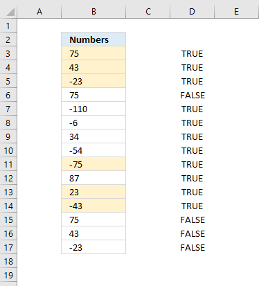
Explaining CF formula in cell B3
COUNTIF($B$3:B3, B3)=1
The first COUNTIF function counts how many values there are in the first argument that match the second argument.
It returns TRUE if it is equal to 1, meaning this is the first instance of the value. In other words, this makes sure that duplicates are not highlighted.
The first argument is also a growing cell reference, the picture below shows what it returns in column D:
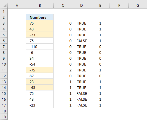
COUNTIF($B$3:B3, B3*-1)
The second COUNTIF function counts how many values there are in the first argument matching B3 but with a different sign, starting from the top.
This verifies that there is a number with a different sign above the current value.
The first argument has a growing cell reference meaning it expands as you copy the formula to cells below. In this case, I am using it as a Conditional Formatting formula, however, it behaves the same.
The picture below shows what it returns in column C:
MATCH(B3*-1,$B$3:$B$17,0)
The MATCH function looks for the number but with a different sign, this verifies it really exists a pair in the first place.
The MATCH function returns a #N/A error if a number is not found
COUNT(MATCH(B3*-1,$B$3:$B$17,0))
The COUNT function then converts error to a 0 (zero). The picture below shows what it returns in column E:
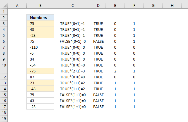
Then the formula adds the numbers in the two last arrays, like this COUNTIF($B$3:B3, B3*-1)+COUNT(MATCH(B3*-1, $B$3:$B$17, 0)
and lastly multiplies with COUNTIF($B$3:B3, B3)=1.
Get Excel *.xlsx file
Matching opposite numbers.xlsx
5. Dynamic conditional formatting
Question: I have a list that I keep adding rows to. How do i create a border that expands as the list expands?
Answer:
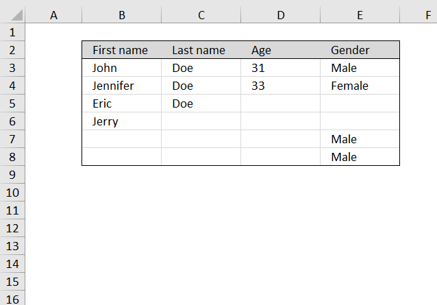
The easiest way to go is an excel defined table, you can customize how it looks easily:
Recommended articles
An Excel table allows you to easily sort, filter and sum values in a data set where values are related.
Adding more rows to your list expands the border automatically. See picture below.

How to create dynamic border
The border on top of the list is static. Here is how to create the top border:
- Select the top cells of your list
- Go to "Home" tab in excel 2007
- Press with left mouse button on the small triangle on the border button in the font window. See picture below.

- Press with left mouse button on "Top border"
The border on the sides of the list is dynamic. Here is how to create the border on the left side:
- Select the leftmost column in your list (In this example C:C)
- Press with left mouse button on "Home" tab on the ribbon
- Press with left mouse button on "Conditional formatting"
- Press with left mouse button on "New rule..."
- Press with left mouse button on "Use a formula to determine which cells to format"
- Press with left mouse button on "Format values where this formula is true" window.
- Type =OR(C1<>"",D1<>"",E1<>"",F1<>"")
- Press with left mouse button on Format button
- Press with left mouse button on "Border tab" tab
- Create a border on left side of cell
- Press with left mouse button on OK!
- Press with left mouse button on OK!
Here is how to create the left and bottom border on the left side:
- Select the leftmost column in your list (In this example C:C)
- Create a new conditional formatting formula. (See above list)
- Type =AND(OR($C1<>"",$D1<>"",$E1<>"",$F1<>""),$C2="",$D2="",$E2="",$F2="")
- Create a border on the left and down side of cell
Do the same thing for the right side (F:F) of the list using the two above examples. Obviously creating borders on the right and down side of cells.
Finally creating the border lines below the list:
- Select the middle columns in your list (In this example D:D and E:E)
- Create a new conditional formatting formula.
- Type =AND(OR($C1<>"",$D1<>"",$E1<>"",$F1<>""),$C2="",$D2="",$E2="",$F2="")
- Create a border on the down side of cell
Get Excel file
create-a-dynamic-border-using-excel-conditional-formatting.xls
(Excel 97-2003 Workbook *.xls)
6. Highlight closest number
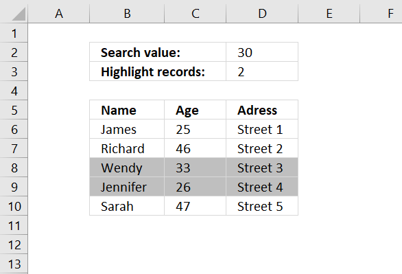
This section demonstrates how to highlight records with the closest value to a criterion, you can also choose to highlight the second closest value (or more).
You can also extract the number using the formula described in this article: Find closest value, perhaps you are also interested in how to find the numbers in a total closest to a given sum.
6.1 Conditional formatting formula
This formula won't work in Excel 2010 and later Excel versions, simply create a named range containing the formula above. Then use that name as the conditional formatting formula, get the file later in this article if you need to see exactly how I did it.
6.2 How to apply conditional formatting formula
Make sure you adjust cell references to your excel sheet.
- Select cells B6:D10
- Press with left mouse button on "Home" tab
- Press with left mouse button on "Conditional Formatting" button
- Press with left mouse button on "New Rule.."
- Press with left mouse button on "Use a formula to determine which cells to format"
- Type =OR(ABS($C6-$C$2)=SMALL(ABS($C$6:$C$10-$C$2), ROW($A$1:INDEX($A:$A, $C$3)))) in "Format values where this formula is TRUE" window.
(The formula displayed in the image above is not used in this article) - Press with left mouse button on "Format.." button
- Press with left mouse button on "Fill" tab
- Select a color for highlighting cells.
- Press with left mouse button on "Ok"
- Press with left mouse button on "Ok"
- Press with left mouse button on "Ok"
6.3 How the conditional formatting formula works in cell C6
Step 1 - Calculate age differences
ABS(number) returns the absolute value of a number, a number without its sign.
ABS($C$6:$C$10-$C$2) returns {5;16;3;4;17}
Step 2 - Create an array with the same size as chosen records to highlight in cell C3.
ROW($A$1:INDEX($A:$A,$C$3))) returns {1;2}
Step 3 - Return the two smallest numbers in array
=OR(ABS($C6-$C$2)=SMALL(ABS($C$6:$C$10-$C$2),ROW($A$1:INDEX($A:$A,$C$3))))
SMALL(array,k) returns the k-th smallest number in this data set.
SMALL(ABS($C$6:$C$10-$C$2),ROW($A$1:INDEX($A:$A,$C$3))) returns {3;4}
Step 4 - Is cell value in C6 equal to any number in array?
=OR(ABS($C6-$C$2)=SMALL(ABS($C$6:$C$10-$C$2),ROW($A$1:INDEX($A:$A,$C$3))))
becomes
OR(logical1, logical2, ...) checks whether any of the arguments are TRUE, and returns TRUE or FALSE. Returns FALSE if only all arguments are FALSE.
$C6 is a relative AND absolute cell reference.
=OR(ABS($C6-$C$2)={3;4}) returns FALSE. Row 6 is not highlighted.
7. Highlight cells based on numerical ranges

This section demonstrates a Conditional Formatting formula that lets you highlight cells based on numerical ranges specified in an Excel Table.
Column A contains numbers from 0 (zero) to 100 in steps of 0.1. Cells in column B are highlighted if the number is inside a range specified in the Excel Table.
For example, cell A1 contains 0 (zero), the corresponding cell B1 is not highlighted. Value 0 (zero) is not in any of the three ranges specified in cell range D4:E6. They are 0.1-0.8, 1.1-1.3, and 1.4-1.6.
I am working on a railway project as planner. How can I create a dynamic strip chart in Excel?
Assume the total length is 10 kilometers and each cell of 100 meters.
If I update the progress from 9.1 km to 9.8 km in the table, how the cell gets highlighted corresponding to the entered chainages.
7.1 Conditional Formatting formula
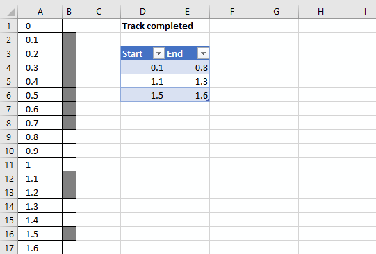
The worksheet above shows you km in column A and corresponding highlighted cells in column B if they are specified in the Excel Table.
You can easily add or remove values to the Excel Table without the need to adjust the conditional formatting formulas.
Conditional formatting formula applied to cell range B1:B101:
7.2 How to create an Excel Table

- Select cell range D3:E6
- Go to tab "Insert" on the ribbon
- Press with left mouse button on the "Table" button
Tip! You can also use the shortcut key CTRL + T to create a table
Excel Tables let you easily organize, filter, and format data on a worksheet. They also let you use structured references that can gro without the need to adjust cell references in a formula.
Learn more about Excel Tables
7.3 How to apply a conditional formatting formula to a cell range

- Select cell range B1:B101.
- Go to tab "Home" on the ribbon if you are not already there.
- Press with mouse on the "Conditional Formatting" button to expand a menu.
- Press with left mouse button on "New Rule..".
- Press with left mouse button on "Use a formula to determine which cells to format".
- Type above formula in dialog box formula bar.
- Press with left mouse button on the "Format..." button.
- Go to tab "Fill".
- Pick a fill color.
- Press with left mouse button on the OK button.
- Press with left mouse button on the OK button.
7.4 Explaining conditional formatting formula
You can't use structured references in a conditional formatting formula unless you use the INDIRECT function for each reference. This applies to Data Validation Lists as well.
Step 1 - Reference an Excel Table in a Conditional Formatting formula

Excel returns an error message if you try to use a reference to an Excel Table in a Conditional Formatting formula.
There is a workaround, simply use the INDIRECT function to make this possible.
Table1[End]
becomes
INDIRECT("Table1[End]")
Step 2 - Check if current cell value is less than the END range values in the Excel Table
(A1<INDIRECT("Table1[End]") returns {TRUE;TRUE;TRUE}
Step 3 - Check if current cell value is greater than or equal to the START values in the Excel Table
A1>=INDIRECT("Table1[Start]" returns {FALSE;FALSE;FALSE}
Step 4 - Multiply arrays
(A1<INDIRECT("Table1[End]"))*(A1>=INDIRECT("Table1[Start]")) returns {0;0;0}
Multiplying boolean values creates integers.
Step 5 - Sum array
SUMPRODUCT((A1<INDIRECT("Table1[End]"))*(A1>=INDIRECT("Table1[Start]"))) returns 0.
0 means False so cell B1 is not formatted gray.
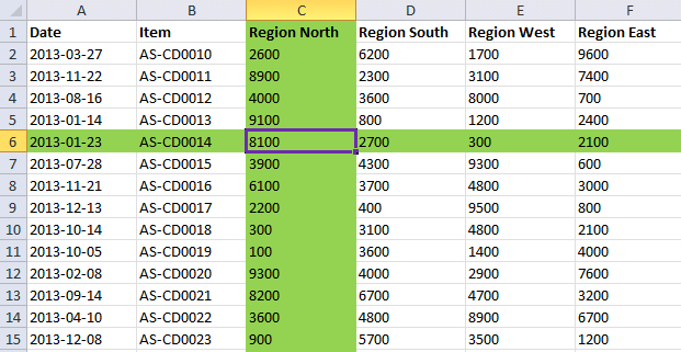
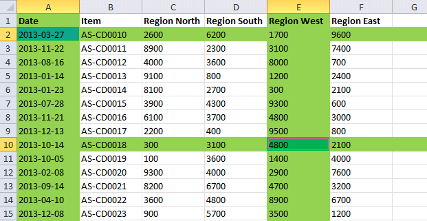
8. How to highlight a row automatically using event macro?
This event code highlights the entire row of the selected cell. I have chosen the color green to highlight the entire row.
How to add code to your workbook
- Press with right mouse button on on the worksheet name and select "View Code". This opens the Visual Basic Editor and the corresponding module.

- Copy the VBA code below and paste it to the module.

- Exit the VB Editor and go back to Excel.
VBA Code
'Eventcode procedure name, you can't change this line
Private Sub Worksheet_SelectionChange(ByVal Target As Range)

'The With ... End With statement allows you to write shorter code by referring to an object only once instead of using it with each property.
'These lines removes cell colors
With Cells.Interior
        .Pattern = xlNone
        .TintAndShade = 0
        .PatternTintAndShade = 0
End With

'These lines applies cell colors to all cells in row of selected cell
With Rows(Selection.Row).Interior
        .Pattern = xlSolid
        .PatternColorIndex = xlAutomatic
        .Color = 5296274
        .TintAndShade = 0
        .PatternTintAndShade = 0
End With
End Sub
Microsoft Docs: Cells | Interior | Pattern | TintAndShade | PatternTintAndShade | PatternColorIndex | Color | Rows
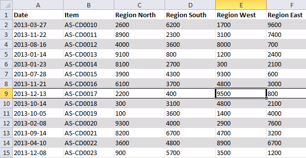
9. Highlight column of the selected cell
This Event code highlights the entire column of the selected cell.
How to add code to your workbook
VBA Code
'Event code
Private Sub Worksheet_SelectionChange(ByVal Target As Range)

'The With ... End With statement allows you to write shorter code by referring to an object only once instead of using it with each property.
'These lines removes cell colors
With Cells.Interior
        .Pattern = xlNone
        .TintAndShade = 0
        .PatternTintAndShade = 0
End With

'These lines applies cell colors to all cells in column of selected cell
With Columns(Selection.Column).Interior
        .Pattern = xlSolid
        .PatternColorIndex = xlAutomatic
        .Color = 5296274
        .TintAndShade = 0
        .PatternTintAndShade = 0
End With

End Sub
Microsoft Docs: Cells | Interior | Pattern | TintAndShade | PatternTintAndShade | PatternColorIndex | Color | Columns | Selection | Selection.Column
10. Highlight row and column of the selected cell
This event code highlights the entire column and row of the selected cell.
How to add code to your workbook
VBA code
'Event code
Private Sub Worksheet_SelectionChange(ByVal Target As Range)

'The With ... End With statement allows you to write shorter code by referring to an object only once instead of using it with each property.
'These lines removes cell colors
With Cells.Interior
        .Pattern = xlNone
        .TintAndShade = 0
        .PatternTintAndShade = 0
End With

'These lines applies cell colors to all cells in row of selected cell
With Rows(Selection.Row).Interior
        .Pattern = xlSolid
        .PatternColorIndex = xlAutomatic
        .Color = 5296274
        .TintAndShade = 0
        .PatternTintAndShade = 0
End With

'These lines applies cell colors to all cells in column of selected cell
With Columns(Selection.Column).Interior
        .Pattern = xlSolid
        .PatternColorIndex = xlAutomatic
        .Color = 5296274
        .TintAndShade = 0
        .PatternTintAndShade = 0
End With

End Sub
Microsoft Docs: Cells | Interior | Pattern | TintAndShade | PatternTintAndShade | PatternColorIndex | Color | Columns | Selection | Selection.Column | Rows | Selection.Row
11. Highlight rows and columns of multiple selected cells
This event code allows you to highlight entire columns and rows of multiple selected cells. Press and hold the SHIFT key to select multiple cells with your mouse.
How to add code to your workbook
'Event code
Private Sub Worksheet_SelectionChange(ByVal Target As Range)


'The With ... End With statement allows you to write shorter code by referring to an object only once instead of using it with each property.
'These lines removes cell colors
With Cells.Interior
        .Pattern = xlNone
        .TintAndShade = 0
        .PatternTintAndShade = 0
End With

'Iterate through all cells in selection
For Each cell In Selection

    'The With ... End With statement allows you to write shorter code by referring to an object only once instead of using it with each property.
    'These lines removes cell colors
    With Rows(cell.Row).Interior
        .Pattern = xlSolid
        .PatternColorIndex = xlAutomatic
        .Color = 5296274
        .TintAndShade = 0
        .PatternTintAndShade = 0
    End With

    'These lines applies cell colors to all cells in column of selected cell
    With Columns(cell.Column).Interior
        .Pattern = xlSolid
        .PatternColorIndex = xlAutomatic
        .Color = 5296274
        .TintAndShade = 0
        .PatternTintAndShade = 0
    End With

    'These lines applies cell colors to all cells in row of selected cell
    With cell.Interior
        .Pattern = xlSolid
        .PatternColorIndex = xlAutomatic
        .Color = 5287936
        .TintAndShade = 0
        .PatternTintAndShade = 0
    End With

Next cell

End Sub
Microsoft Docs: Cells | Interior | Pattern | TintAndShade | PatternTintAndShade | PatternColorIndex | Color | Columns | Selection | Rows
12. Apply borders to the row of the selected cell
This event procedure applies borders to the row. It does not remove colors from cells instead it removes all borders every time you select a new cell.
How to add code to your workbook
'Event code
Private Sub Worksheet_SelectionChange(ByVal Target As Range)


'The With ... End With statement allows you to write shorter code by referring to an object only once instead of using it with each property.
'These lines removes cell colors
With Cells
    .Borders(xlDiagonalDown).LineStyle = xlNone
    .Borders(xlDiagonalUp).LineStyle = xlNone
    .Borders(xlEdgeLeft).LineStyle = xlNone
    .Borders(xlEdgeTop).LineStyle = xlNone
    .Borders(xlEdgeBottom).LineStyle = xlNone
    .Borders(xlEdgeRight).LineStyle = xlNone
    .Borders(xlInsideVertical).LineStyle = xlNone
    .Borders(xlInsideHorizontal).LineStyle = xlNone
End With

'These lines enables a top cell border to all cells in row of selected cell
With Rows(Selection.Row).Borders(xlEdgeTop)
        .LineStyle = xlContinuous
        .ColorIndex = 0
        .TintAndShade = 0
        .Weight = xlThin
End With

'These lines enables a bottom cell border to all cells in row of selected cell
With Rows(Selection.Row).Borders(xlEdgeBottom)
    .LineStyle = xlContinuous
    .ColorIndex = 0
    .TintAndShade = 0
    .Weight = xlThin
End With

End Sub
Microsoft Docs: Cells | Interior | Pattern | TintAndShade | PatternTintAndShade | PatternColorIndex | Color | Columns | Selection | Rows | Cells.Borders | LineStyle
13. Dowmload macro-enabled Excel file * .xlsm
Recommended reading
Built-in conditional formatting
Data Bars Color scales IconsHighlight cells rule
Highlight cells containing stringHighlight a date occuring
Conditional Formatting Basics
Highlight unique/duplicates
Top bottom rules
Highlight top 10 valuesHighlight top 10 % values
Highlight above average values
Basic CF formulas
Working with Conditional Formatting formulasFind numbers in close proximity to a given number
Highlight empty cells
Highlight text values
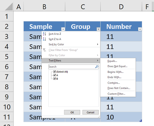
Search using CF
Highlight records – multiple criteria [OR logic]Highlight records [AND logic]
Highlight records containing text strings (AND Logic)
Highlight lookup values
Unique distinct
How to highlight unique distinct valuesHighlight unique values and unique distinct values in a cell range
Highlight unique values in a filtered Excel table
Highlight unique distinct records
Duplicates
How to highlight duplicate valuesHighlight duplicates in two columns
Highlight duplicate values in a cell range
Highlight smallest duplicate number
Highlight more than once taken course in any given day
Highlight duplicates with same date, week or month
Highlight duplicate records
Highlight duplicate columns
Highlight duplicates in a filtered Excel Table
Compare
Highlight missing values between to columnsCompare two columns and highlight values in common
Compare two lists of data: Highlight common records
Compare tables: Highlight records not in both tables
How to highlight differences and common values in lists
Compare two columns and highlight differences
Min max
Highlight smallest duplicate numberHow to highlight MAX and MIN value based on month
Highlight closest number
Dates
Advanced Date Highlighting Techniques in ExcelHow to highlight MAX and MIN value based on month
Highlight odd/even months
Highlight overlapping date ranges using conditional formatting
Highlight records based on overlapping date ranges and a condition
Highlight date ranges overlapping selected record [VBA]
How to highlight weekends [Conditional Formatting]
How to highlight dates based on day of week
Highlight current date
Misc
Highlight every other rowDynamic formatting
Advanced Techniques for Conditional Formatting
Highlight cells based on ranges
Highlight opposite numbers
Highlight cells based on coordinates
Excel categories
39 Responses to “Advanced Techniques for Conditional Formatting”
Leave a Reply
How to comment
How to add a formula to your comment
<code>Insert your formula here.</code>
Convert less than and larger than signs
Use html character entities instead of less than and larger than signs.
< becomes < and > becomes >
How to add VBA code to your comment
[vb 1="vbnet" language=","]
Put your VBA code here.
[/vb]
How to add a picture to your comment:
Upload picture to postimage.org or imgur
Paste image link to your comment.
This is helpful, thanks, but I've been looking for the formatting to take place AS I fill new cells.
So my scenario is: A clear-formatted excel sheet, and ONCE you insert data into each row, the color of the row changes, e.g. row 1 becomes light blue, row 2 becomes dark blue, BUT row 3 is still clear-formatted because I haven't inserted data in it yet.
Do you know how I can do that?
*Thanks!!!*
@Sawsan,
Select all the cells (starting from upper left corner of the range so the the upper left cell ends up the active cell) that you think you will ever need to put your alternating row colors in (I would refrain from selecting entire columns), then follow the blog's instructions to get to the Conditional Formatting dialog box and then use this formula...
=AND(ISEVEN(ROW()),COUNTIF($A1:$C1,"*")>0)
Change the range as indicated, but note that your formula should only specify the first row's cells range even though you will have many more rows selected.
@Sawsan,
I guess I missed your request for a second color. That will require a second condition for the second color... use the identical formula I gave you in my previous message for this condition, but change the ISEVEN function to ISODD.
hi,
i'm interested to know on the conditional formatting.
how do i set the condition to evaluate a dynamic range?
my example is this:
Rule: =MAX($G$5:$G$20)=$G5
Applied to: =$AG$5:$AG$20
based on the value in G5:G20, the rule will determine the max value and highlight it on AG5:AG20
If i add new rows of data to G21 onwards, the rules does not "extend" to the newly added rows.
david,
I got this working in excel 2007:
Rule: =MAX(OFFSET($G$5;0;0;COUNTA($G5:$G1000))=$G5
Applied to: =OFFSET($AG$5;0;0;COUNTA($G5:$G1000)
thanks oscar,
i was using a dynamic named range as the rule in conditional formatting.
will try ur solutions ;)
thanks!!!
Hi! you can go here to know how to make conditional lists:
https://runakay.blogspot.com/2011/03/conditional-lists-on-excel.html
Thanks!
I duplicated the spreadsheet but the formula did not work for me on Excel 2007. It says there's an error. Could you check and explain? Thx.
Lyon,
You probably have to adjust cell references in conditional formatting formula to your spreadsheet.
As I mentioned, I recreate the sample spreadsheet and copy paste the formula. But Excel 2007 says there's an error in the formula. Something is not right.
Lyon,
You are right, I found errors. I have corrected them.
Thanks for pointing them out.
It's now working! Great! Thanks a lot for your quick response.
Absoultely great
only small problem
when I enter value of 40 in search value in example given
it highlights 3 values (wendy also) I accepted it to highlight
only richard & sarah
draw a border line automatically in a cell with fomula of anather cell
Something doesn't work quite right with the above and below average conditional formattings.
Brilliant nonetheless.
At least not in the version I opened and ran on Excel 2010
Cape,
Something doesn't work quite right with the above and below average conditional formattings.
What happens, what is wrong? I have excel 2010.
Great job and is very useful
Thank you very much Mr. (Oscar)
Thank you!
Work more than wonderful, because you are a wonderful person
Dear Oscar
I want to highlight the row if the checkbox in my customized menu is pressed on.
please help & provide code.
Dear Oscar
In your first example Excel highlights all rows until last column (XFD). I need highlight from column A to column R. Is it possible?
Thanks!
Hi Oscar,
Thanks a lot for all these wonderful macros.
I wanna know how the codes will be if I want to maintain the headers with blue color and the color changes happens only to the cells below the header.
hello
I want program with VBA
with press with left mouse button on a picture count into cell
thanks
Hi Oscar,
Is it possible to highlight a row but only within a table?
Thanks
Nilhan
Hi Oscar,
First i want to tell you Big Thank You for these examples and working codes.
I would like to as, is there a way to maintain all other colors on my sheet and still get benefit from "Highlight row and column"/code/?
If you can just send me this tipe of code on my email i will be very thankful.
BR,
Martin
I used this formula, however, I received errors. I see this post is quite old. is there an updated formula for excel 2010?
kris
You are right, it is not working for excel 2010.
I created a named range with the same formula and used that named range in a CF formula.
Please can you elaborate as to how to get this done in excel 2013.
Ranjan
See my answer to kris above, it should work in excel 2013 also?
HI,
I tried your formula to do a custom border but in vain.
I have a fiscal Year period from data source which user selects number of months.. if it is for 2016 then 12 months and for 2017 2 months.
Somehow I couldn't able to follow your steps.
In your excel the data starts from C5 WHERE AS c4 IS Header.. I'm not sure why C1.
Can you please help?.
Thanks,
Jothi
Jyothi
The CF formulas are applied to whole columns. Example, column C starts with cell C1 so the CF formula must start with cell C1.
Dear Sir.
Big thanks for examples and working codes is very useful
please explan how to change colour
Sanjaya
Sanjaya,
I believe you change this:
Interior.Color property (Excel)
Thanks a lot for your sharing.
How can we use this as default in excel?
Zin Thida Win
You can save it to your personal workbook and always have access to it.
Copy your macros to a Personal Macro Workbook
Add your personal Excel Macros to the ribbon
How can I copy this conditional formatting formula to other cells WITHOUT having to adapt the $cells?
Is there any option to use the highlighting formular with a relative cell reference? This would make it much easier to copy the format...
Best regards,
Franz
Franz,
To change the range of cells that the conditional formatting rules applies to: https://spreadsheeto.com/conditional-formatting/#editingrule