Extract a unique distinct list from multiple non adjacent cell ranges
Question: I have two ranges or lists (List1 and List2) from where I would like to extract a unique distinct list? Merge two lists without duplicates, in other words.
What's on this page
- List unique distinct values in two columns - Excel 365
- List unique distinct list values in two columns - earlier version 1
- List unique distinct list in two columns - earlier version 2
- List unique distinct values in two columns, no blanks
- Get Excel *.xlsx file
- Extract a unique distinct list from three columns
- Extract a unique distinct list from three columns - Excel 365
- Extract a unique distinct list from three columns with possible blanks
- Extract a unique distinct list from three columns with possible blanks - Excel 365
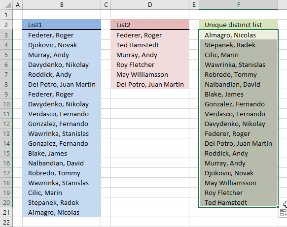
1. Extract a unique distinct list from two columns - Excel 365

Excel 365 dynamic array formula in cell F3:
Explaining formula in cell F3
Step 1 - Combine cell ranges
The comma is a union operator in Excel, it lets you combine multiple cell ranges, however, most Excel functions don't let you do that.
The TOCOL function is one of few functions that let you combine multiple cell ranges, the parentheses are needed in order to not confuse the TOCOL function. Remember the comma is used to separate arguments in Excel functions.
The TOCOL function returns a #VALUE! error if you forget the parentheses, the reason is that the TOCOL function interprets the comma as a delimiter for arguments.
(B3:B21,D3:D8)
Step 2 - Rearrange values to a single column
The TOCOL function rearranges values in 2D cell ranges to a single column.
Function syntax: TOCOL(array, [ignore], [scan_by_col])
TOCOL((B3:B21,D3:D8))
returns {"Federer, Roger "; "Djokovic, Novak "; "Murray, Andy "; ... ; "Del Potro, Juan Martin "}
Why not use the VSTACK function? The TOCOL function has some great features that the VSTACK function is lacking, it lets you ignore blanks and error values. The second argument lets you specify these options.
Step 3 - Extract unique distinct values
The UNIQUE function returns a unique or unique distinct list.
Function syntax: UNIQUE(array,[by_col],[exactly_once])
UNIQUE(TOCOL((B3:B21,D3:D8)))
returns {"Federer, Roger "; "Djokovic, Novak "; "Murray, Andy "; ... ; "May Williamsson"}
2. Extract a unique distinct list from two columns - earlier version 1
Update! 2017-09-01, smaller regular formula in cell F3:
2.1 Watch a video explaining the formula
2.2 Explaining regular formula in cell F3
This formula consists of two similar parts, one returns values from List1 and the other returns values from List2.
Step 1 - Prevent duplicate values
The COUNTIF function counts values based on a condition, in this case, I am counting values in cells above. This makes sure that duplicates are ignored.
COUNTIF($F$2:F2,$B$3:$B$21)=0
returns {TRUE;TRUE;TRUE; ... ;TRUE}
Step 2 - Divide 1 with array
The LOOKUP function ignores error and if we divide 1 with 0 an error occurs. 1/0 = #DIV/0!
1/(COUNTIF($F$2:F2,$B$3:$B$21)=0)
returns {1;1;1;... ;1}
Step 3 - Return value based on array
LOOKUP(2, 1/(COUNTIF($F$2:F2,$B$3:$B$21)=0), $B$3:$B$21)
returns Almagro, Nicolas in cell F3.
Step 4 - Return values from List2
When values run out from List1 formula1 returns errors, the IFERROR function then moves to formula2.
IFERROR(formula1, formula2)
formula2 is just like formula1 except that it returns values from List2.
Array formula in F3:
2.3 How to create an array formula
- Select cell C2
- Press with left mouse button on in formula bar
- Paste array formula to formula bar
- Press and hold Ctrl+ Shift
- Press Enter
- Release all keys
Recommended article
Recommended articles

Array formulas allows you to do advanced calculations not possible with regular formulas.
2.4 How to copy formula
- Copy cell C2
- Select cell range C3:C19
- Paste
3. Extract a unique distinct list from two columns - earlier version 2

Array formula in cell C2:
Get excel *.xls file
how-to-extract-a-unique-distinct-list-from-two-columns-in-excel-2003.xls
(Excel 97-2003 Workbook *.xls)
4. Unique distinct values from two columns, no blanks
6. Extract a unique distinct list from three columns
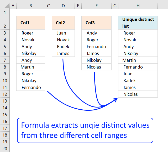
The image above shows three different cell ranges populated with names, they are B3:B11, D3:D6, and F3:F8. The following formula works in all versions, however, I recommend Excel 365 users to go with the much smaller and easier formula in section 2.
It extracts unique distinct values from all three cell ranges B3:B11, D3:D6, and F3:F8 combined. Unique distinct means that only one instance is extracted even if there are duplicates in the data source ranges. Note that this formula does not differentiate between upper and lower case letters. In other words, A and a is the same value and a is considered a duplicate in this case.
Formula in H3:
This formula consists of three similar parts, one returns values from Col1, the second one from col2 and the third from Col3. The formula detects when values from one cell range has all been displayed and continues to the next cell range. This is made possible using the IFERROR function in three nested configurations. Two IFERROR functions are required as there are three columns. The last argument in the first IFERROR function extracts unique distinct values from the last source data range.
IFERROR(IFERROR(formula1, formula2), formula3)
This formula has issues if the source data ranges contain blank empty cells, section 3 demonstrates another formula that takes care of this issue.
6.1 Explaining formula in cell H3
Step 1 - Prevent duplicate values
The COUNTIF function counts values based on a condition, in this case, I am counting values in the cells above. This makes sure that duplicates are ignored.
COUNTIF($H$2:H2,$B$3:$B$11)=0
returns {TRUE;TRUE; ... ; TRUE}
Step 2 - Divide 1 with array
The LOOKUP function ignores errors and if we divide 1 by 0 an error occurs. 1/0 = #DIV/0!
1/(COUNTIF($F$2:F2,$B$3:$B$11)=0)
returns {1;1;... ;1}
Step 3 - Return value based on the array
LOOKUP(2, 1/(COUNTIF($F$2:F2,$B$3:$B$11)=0), $B$3:$B$11)
returns " Fernando " in cell F3.
Step 4 - Return values from Col2
When values run out from Col1 formula1 returns errors, the IFERROR function then moves to formula2.
IFERROR(IFERROR(formula1, formula2), formula3)
formula2 is just like formula1 except that it returns values from Col2 etc.
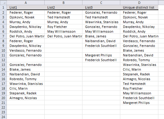
7. Extract a unique distinct list from three columns - Excel 365

The image above shows three different cell ranges in cells B3:B21, D3:D8, and F3:F13. The Excel 365 formula extracts unique distinct values from three cell ranges combined. The result is an dynamic array that spills to cell H3 and cells below as far as needed. The formula is entered as a regular formula despite the fact that the formula is an Excel 365 dynamic array formula.
Excel 365 dynamic array formula in cell H3:
This formula is not considering upper and lower case letters as different values, in other words, A and a is the same value. You need a different formula that probably uses the EXACT function to differentiate between values with upper and lower case letters.
Here is a quick break-down of what the formula above does:
- (B3:B21,D3:D8,F3:F13): Some functions but not all allows you to combine cell references. This is how you do that.
- TOCOL((B3:B21,D3:D8,F3:F13)): Rearrange values so that they fit one column wide.
- UNIQUE(TOCOL((B3:B21,D3:D8,F3:F13))): Extract unique distinct values.
This formula has issues if the source data ranges contain blank empty cells, section 4 demonstrates what you need to change in order to take care of this issue. The following section 2.1 explains the formula in greater detail.
7.1 Explaining formula
Step 1 - Merge cells
Some Excel functions allow you to combine multiple cell ranges in one argument, the TOCOL function is one of those functions.
(B3:B21,D3:D8,F3:F13)
Step 2 - Rearrange values
The TOCOL function rearranges values in 2D cell ranges to a single column.
Function syntax: TOCOL(array, [ignore], [scan_by_col])
TOCOL((B3:B21,D3:D8,F3:F13))
returns
{"Federer, Roger "; "Djokovic, Novak "; ... ; "Frederick Southbell"}
Step 3 - List unique distinct values
The UNIQUE function returns a unique or unique distinct list.
Function syntax: UNIQUE(array,[by_col],[exactly_once])
UNIQUE(TOCOL((B3:B21,D3:D8,F3:F13)))
becomes
UNIQUE({"Federer, Roger "; "Djokovic, Novak "; ... ; "Frederick Southbell"})
and returns
{"Federer, Roger "; "Djokovic, Novak "; ... ; "Margeret Philips"}
8. Extract a unique distinct list from three columns with possible blanks
The image above shows three different cell ranges A2:A20, B2:B7, and C2:C12. The first and last cell range has empty blank cells that the following formula takes care of. The following formula works in all versions, however, I recommend Excel 365 users to go with the much smaller and easier formula in section 4.
Array formula in D2:
The formula in cell D2 extracts unique distinct values from A2:A20, B2:B7, and C2:C12 and ignores possible blank values. This formula is not considering upper and lower case letters as different values, in other words, A and a is the same value.
How to enter an array formula
- Select cell D2
- Press with left mouse button on in formula bar
- Paste array formula to formula bar
- Press and hold CTRL + SHIFT
- Press ENTER
9. Extract a unique distinct list from three columns with possible blanks - Excel 365

Excel 365 dynamic array formula in cell H3:
Check section 2 above for how the formula works.
Get Excel *.xlsx file
how-to-extract-a-unique-list-from-three-columns-in-excelv3.xlsx
Unique distinct values category

First, let me explain the difference between unique values and unique distinct values, it is important you know the difference […]
This article demonstrates Excel formulas that allows you to list unique distinct values from a single column and sort them […]
This article shows how to extract unique distinct values based on a condition applied to an adjacent column using formulas. […]
Excel categories
122 Responses to “Extract a unique distinct list from multiple non adjacent cell ranges”
Leave a Reply
How to comment
How to add a formula to your comment
<code>Insert your formula here.</code>
Convert less than and larger than signs
Use html character entities instead of less than and larger than signs.
< becomes < and > becomes >
How to add VBA code to your comment
[vb 1="vbnet" language=","]
Put your VBA code here.
[/vb]
How to add a picture to your comment:
Upload picture to postimage.org or imgur
Paste image link to your comment.
hello,
i´m looking for a solution for this problem (with 7 cols) for excel 2003. One problem: the lists in the columns sometimes have empty cells in between.
Hope you can help...
Thank you
Harold
Hello Harold!
I think that would require vba. Post your question in a forum like https://www.excelforum.com/. I am sure they can help you.
Thank you for your comment!
/Oscar
I need to improve my vba skills...
Harold,
Maybe this blog post can help you?
https://www.get-digital-help.com/extract-a-unique-distinct-list-sorted-alphabetically-removing-blanks-from-a-range-in-excel/
Can you please post an Excel 2003 sample of this. The 2003 formula does not work.
Thanks
No problem Rav!
I have now attached an excel 2003 file to this blog post.
Hello - trying to use this formula on a spreadsheet (Excel 2007) very similar to the one you show in your screenshot. I'm getting no values returned, so tried to get your example file and instead of an .xlsx file I received a zip file that contains a bunch of .xml files. The 2003 example file is fine ...
Thanks for posting this!
OK, I manaaged to use the 2003 formula in my Excel 2007 and it works ... right down to cell C24. After that I get a "Value not available error". I see that your example is only 24 rows long, but I don't see anywhere in the formula that it specifies to stop at row 24. If I continue copy/pasting the formula in cells 25 and below, shouldn't it use relative formatting to adjust properly?
David,
I tried the .xlsx file and it works fine here.
I am not sure I understand but I´ll give it a try:
The relative reference should adjust properly. But if you add more values to any of the lists, the named ranges are not dynamic. You need to change the named ranges to include the new values.
Thank you for this guide! Really helpful!
Although is it possible to extract an unique distinct list from three columns?
Eduardo Ristow,
Extract a unique distinct list from three columns in excel
Hi Oscar
I can't get these formulas running on excel 2010
I have two columns (A and B) with server names and I need unique values in column C. And is it possible to get unique names from different sheets (column A in sheet one contains server names from one automatic export and column A in sheet two contains server names from another automatic export) and I would need unique values in sheet 3.
Best regards
hrvoje,
The attached file contains three sheets.
Sheet 3 extracts values from column A in sheet 1 and 2.
Sheet 1 contains a dynamic range: =OFFSET(Sheet1!$A$2,0,0,COUNTA(Sheet1!$A$2:$A$10000))
Sheet 2 contains a dynamic range: =OFFSET(Sheet2!$A$2,0,0,COUNTA(Sheet2!$A$2:$A$10000))
You may have to adjust cell references in both dynamic ranges. Remember, the formulas can´t process blank cells.
Get the Excel *.xslx file
how-to-extract-a-unique-list-from-two-columns-in-different-sheets-in-excel-2007-dynamic-ranges1.xlsx
Hi Oscar. Thank you very much for your fast response.
When I press with left mouse button on a link I get error "Sorry, but you are looking for something that isn't here."
And if I have 3 sheets with data then I just add another sheet and paste formula =OFFSET(Sheet3!$A$2,0,0,COUNTA(Sheet1!$A$2:$A$10000))?
Best regards,
Hrvoje
hrvoje,
thanks, it works now!
And if I have 3 sheets with data then I just add another sheet and paste formula =OFFSET(Sheet3!$A$2,0,0,COUNTA(Sheet1!$A$2:$A$10000))
Yes. You need a larger array formula, see my attached file to Eduardo Ristow.
Dear, Oscar,
I have a two ranges/lists. How to extract the same values from other range contained in two ranges (without VBA)?
Can you help?
Rita,
unique-distinct-and-common-values-from-two-ranges.xls
That is what I wanted.
Thanks for your quick reply, Oscar!
Rita.
Oscar,
Could you modify you formula to use it with criterion?
e.g. - criterion for GG and II from your reply is QWERTY in A:A column, bun in B:B are other criteria in coincidence with one II.
Can you help?
Rita,
I am not sure I understand. Can you provide an example and desired outcome?
UNIQUE DISTINCT AND COMMON VALUES FROM TWO RANGES USING CRITERION
CRITERIA List1 CRITERIA List2 Common values with criterion:
for for
list 1 list2
other AA QWERTY GG GG
other BB other HH JJ
other CC other II #error!
QWERTY GG QWERTY JJ
other EE other KK
other FF other LL
other GG other MM
other HH other YY
QWERTY II other OO
QWERTY JJ other PP
Thank's.
Ohh, sorry!
Another stucture when posting.
Rita,
See attached file:
unique-distinct-and-common-values-from-two-ranges.xlsx
Not exactly, Oscar.
Because the G:G range didn't exclude HH value (HH="other").
What I want it so that the G:G range only have a values with QWERTY criterion.
Thanks anyway.
But you're still help me?
Rita,
See attached file:
unique-distinct-and-common-values-from-two-ranges1.xlsx
Yes, thank you, Oscar!
Hi, Oscar!
If we replace this part *(COUNTIF($J$1,$A$2:$A$11)>0) of the formula by *(IF($J$1=$D$2:$D$11,ROW($E$2:$E$11))), formula will work more correctly with big ranges.
Oscar, I need your help.
How to modify this formula - {INDEX($E$2:$E$11,MATCH(0,COUNTIF($G$1:G1,$E$2:$E$11)+COUNTIF($B$2:$B$11,$E$2:$E$11),0))} that it works with criterion "OTHER" from your last attached example file? I need values from List2 with "other" criterion are not in List1 with "other" criterion.
The rusult is II. Because in List2 II with "other" criterion, but in List1 II with "QWERTY" criterion, that's what I want - II.
Can you help?
Rita,
Your question is really interesting! But I have no answer! That makes it even more interesting.
Thanks anyway, Oscar.
I have two columns containing data as follows,
ISSUE TENOR
06-Sep-12 84
06-Sep-12 84
20-Sep-12 84
20-Sep-12 84
04-Oct-12 84
04-Oct-12 84
06-Sep-12 182
06-Sep-12 182
06-Sep-12 182
20-Sep-12 182
20-Sep-12 182
04-Oct-12 182
04-Oct-12 182
06-Sep-12 364
06-Sep-12 364
06-Sep-12 364
20-Sep-12 364
20-Sep-12 364
26-Jul-12 364
04-Oct-12 364
04-Oct-12 364
Formual should show the following result:
ISSUE TENOR
06-Sep-12 84
20-Sep-12 84
04-Oct-12 84
06-Sep-12 182
20-Sep-12 182
04-Oct-12 182
06-Sep-12 364
20-Sep-12 364
26-Jul-12 364
04-Oct-12 364
I want a unique list of ISSUE dates falling in all three tenors of 84, 182, and 364 days.
Please tell me the formula to reslove my query.
Your help shell be highly appricated.
Nadeem,
Muhammad Nadeem Bhatti,
Read this post:
Filter unique distinct row records in excel 2007
Thanks a lot sir. Surely, you are a great teacher.
(Oscar)
Nadeem,
Sir, Please tell me how to sort on date and tenor.
Look forward to your reply.
Regards,
Nadeem Bhatti.
Muhammad Nadeem Bhatti,
I think you have to copy the values returned from the array formula to a new sheet and then sort on date and tenor.
Perhaps this post is interesting:
Sort values in parallel (array formula)
Thanks Oscar. I've just used this and saved myself a whole load of manual work.
trumpet,
Thank you for commenting!
You are a Prince among men!
WOW you saved me ALL kinds of excel Hell.
I have been pulling my hair out, looking for this solution for years...
You are still a GOD.
But I am having a problem...
The unique list works (I think), but after that I am trying to use the list in a Vlookup and hitting a bug I cannot figure out...
Any chance I could email you a file to have a quick look?
Many thanks! (You have my email...)
Careyz,
You can upload the file here.
OK I uploaded a file for you.
Did you get it?
You can reply here or maybe better to my email.
[...] this VBA method.... Atlas: Excel Training | Testing | Consulting And a formula solution here.... Extract a unique distinct list from three columns in excel | Get Digital Help - Microsoft Excel reso... This is the result of the formula, it's not perfect (I can't get rid of the 0) and the result is [...]
Muhammad Nadeem Bhatti,
I think you have to copy the values returned from the array formula to a new sheet and then sort on date and tenor.
Perhaps this post is interesting:
Sort values in parallel (array formula)
Reply
Hi Again,
Thanks for your help as above.
Is there any possibility to sort the values in side the primary array formula. Basically I want to avoid copy paste and add another work sheet to save my time.
Look forward to your reply on this.
Thanks and Regards,
Muhammad Nadeem.
Muhammad Nadeem Bhatti,
Sorting multiple columns using array formulas is complicated.
I recommend creating a macro that automatically copy and paste your values.
Oscar,
Using two columns in tables - How do I remove the blanks within this solution?.
Thanks - Alex
Alex,
Array formula:
See this comment
Oscar,
This works like a charm..
Appreciate the help - Alex
I cannot get this formula to work at all. Not being really that familiar with more complex Excel functionality, what is the logic of the formula? (I am using Excel 2003.)
Maddy Eid,
What happens? #NAME? error?
Here is an explanation of the formula:
How to extract unique distinct values from a column
Hi Oscar,
#Name if I haven't set up names, #N/A if I set up names or replace the name by the column reference $A:$A... As the lists are dynamic, I'd prefer not to use names wherever possible.
Thanks,
Maddy
Maddy Eid,
I am not sure why you get #N/A but I recommend converting the list to defined table. Tables are dynamic and easy to reference. I believe there is a similar feature in excel 2003: List
https://www.contextures.com/xlExcelTable01.html
A cell reference to the entire column A makes the array formula very slow.
Hi Oscar,
I'd better explain what I'm trying to achieve: we have a project that set up teams to deliver a specific short term service and we are trying to see the effect on the subsequent requirement for long term services or another episode of short term care after each short term service episode. However, people can have multiple episodes of each of the short and/or long term services, which means I need to end up with a flat file of all services sorted by client ID, then the service start date with the short term episode number and all service episode number. From that, I can create pivot tables detailing length of time it takes to start a long term service after the short term service.
So, I have 3 different data extracts:
* Historic Short Term (up to end of the last financial year) refreshed 2-3 times per year
* Current Short Term (from the start of the current financial year) refreshed every 6 weeks or so
* Long Term refreshed when I update the Excel
However, the Short term extracts overlap by about 3 months each way (no, I didn't set these up and I have no control over what is extracted - it's something horrible involving Oracle tables which IT handles), so I only take episodes terminated up to the end of the last financial year from the Historic data, and all episodes from the Current data (and I'll start missing historic terminations until the Historic data is updated). These I need to combine into a single file, sorted by client ID and service start date from which I create the short term episode number by date.
Once I have done that, I then need to slot in the long term services, but only for those clients receiving a short term service (about 12,000 clients get long term services and about 3,000 have had a short term service). Again, I need to sort the file by client ID and service start date from which I create the any service episode number by date; but the short term service episode numbers must remain static as I am only interested in what is the next service following any short term termination and how long it is until the start of that service.
From that, I create the various pivot tables. Basically, it can be broken into 2 problems: combining the short term data into a single file, then appending the long term data where a client has had short term services. If I have to end up creating an enormous file of all services regardless of whether the client has had a short term service or not, then I will, but I think my boss wants me to do it all in Excel and not use Business Objects (which is my preferred solution).
Maddy Eid,
Can you provide some fake example data and the desired outcome?
Dear Oscar,
I got some data to be sorted.
I have data in below formate
Column -1 Column - 2
[email protected] 1
[email protected] 2
[email protected] 3
[email protected] 4
[email protected] 5
[email protected] 1
[email protected] 2
[email protected] 3
[email protected] 4
[email protected] 5
I want this data in below format
[email protected] 1 2 3 4 5
[email protected] 1 2 3 4 5
Can you please help me to sort this?
Thanks in advance Oscar, Ravi
Ravi,
Array formula in cell B14:
=INDEX($B$3:$B$12, MATCH(0, COUNTIF($B$13:B13, $B$3:$B$12), 0))
Array formula in cell C14:
=INDEX($C$3:$C$12, SMALL(IF(COUNTIF($B14,$B$3:$B$12), MATCH(ROW($C$3:$C$12), ROW($C$3:$C$12)), ""), COLUMN(A1)))
Get the Excel *.xlsx file
Ravi.xlsx
[...] Oscars formulas. Thanks for your response Robert, I have visited the web site you given, I found Extract a unique distinct list from three columns,But this is not what I want, but I will try Pivot Table and again thanks for your [...]
Hi Oscar,
First of all, thank you for all the great formulas you have posted on this website, it has helped me alot.
I am using the formula above to extract a unique list from two columns. It is working great, except from one small detail which I can't figure out. When I add two or more dates, all are shown in the result column. But when I only have one value in one column, the result column is empty. Do you know what can cause this?
I have uploaded a test file here if you have the time to investigate it:
https://sprend.com/download.htm?C=e30a0e307afb448389a240d69fc7d9ce
Thanks in advance.
Best Regards,
Viktor
Viktor,
It seems that MATCH(0,COUNTIF($C$2:C2,OFFSET($A$1,2,0,COUNTA($A:$A)-2,1))+0,0) returns #N/A.
I converted your dynamic cell ranges to excel defined tables but that didn´t solve it.
Hi Oscar,
Thank you for your reply. So you don't have any idea how it can be solved? Do you have any alternate solution that I can try?
Regards,
Viktor
Viktor,
I remember someone asking the same question and posted a solution. I can´t find the comment.
I have a data set that is a combination of date and a unique id from 2 sources in 2 separate columns , and each day the data gets bigger up to a maximum of 3000 lines how would would i use this formula to list the unique value from these lists, compensating for the blacks as the next they will have data in them in EXCEL 2010?
Many Thanks
James Jones
Meant Blank cells not blacks.
RJJ
RJJ,
See this post: Filter unique distinct row records in excel 2007
Oscar,
Another question relating to my prior 'table question'. I may have a couple of rows that are blank in my first column of data. The index column is then returning a blank in the indexed column. Is there anyway to remove this?.
Thanks,
Alex
Oscar,
To specify, the blank lines in row 2 and 3 after the header.
Thanks,
Alex
Alex,
My previous comment to you seems to be wrong.
New array formula:
=IFERROR(IFERROR(INDEX(Table1[Name], MATCH(0, COUNTIF($G$1:G1, Table1[Name])+(Table1[Name]=""), 0)), INDEX(Table2[Name], MATCH(0, COUNTIF($G$1:G1, Table2[Name])+(Table2[Name]=""), 0))), "")
Get the Excel *.xlsx file
how-to-extract-a-unique-list-from-two-columns-in-excel-2007-Alex.xlsx
Oscar,
I believe - that has it. I have been using this in conjuction with some automated reports out of system and blanks are an issue, as I limit the data..
Thanks for all the help.
Alex
Hi Oscar,
I am really amazed to see your examples in the thread "Extract a unique distinct list from three columns with possible blanks". However, Do you have the working example file for excel 2003 version? I tried to manipulate your formula used in excel 2007 but failed to get the result. Appreciate if you can share one please.
Regards,
vidya
Vidya Shankar,
how-to-extract-a-unique-list-from-three-columns-in-excelv2-excel-2003.xls
[...] know that this problem could be solved via formula at all, but the client provided me a helpful link (thanks Oscar), which guided me to working [...]
Hi
wondering if you can help...
i have several columns of data (over 100 rows) of which some are blanks others have data within them.
i want to create a new column by looking at each row of data, for which there could be a result of 4 options.
20C BB 21C BBC 21C BBF ETH PS GENERAL NEW RESULT
YES DATA
NONE
NONE
YES GENERAL
YES DATA
YES GENERAL
YES YES BOTH
YES DATA
NONE
NONE
YES GENERAL
YES BB
YES BB
in the above there are 6 colums of data....i want to the new result list.
Criteria is
if YES is in columns A,B or C = BB
if YES is in columns D or E = DATA
if YES in column F = GENERAL
if Blank in all columns = NONE
can you help with this please???
Thanks
sofie,
Get the Excel *.xlsx file
sofie.xlsx
Hi Oscar,
I really like your formula, except for a tiny little problem. What if I don't know how many to copy or drag down? is there a way to automate this and include it in the formula? for example I have 864 rows in column A and 958 rows in column B but I don't know how many of A and B would make column C....
Patrick Wiegering,
What if I don't know how many to copy or drag down? is there a way to automate this and include it in the formula?
Not that I know of.
How do you do with multiple columns? I have 3, but I wonder what if there is more? Just add iferror??
Sebastian,
Yes!
https://www.get-digital-help.com/extract-a-unique-distinct-list-from-three-columns-in-excel/
How do you extract a unique distinct alphabetised list?
john dalton,
Read this:
Create a drop down list containing only unique distinct alphabetically sorted text values using excel array formula
Oscar, thank you! You really seem to have solution to everything, nice!
My case is a little different. I spent more than 5 hours to find an answer but I must ask directly, so people like you might enlight me.
I have 2 columns:
Column A: standardized list of values (acronyms)
Column B: check list (I put an "x" for the values in Column A whcih I want to have them in a dynamic named range). This column, as you can figure out, contains blank cells.
How do I define the Named range formula so I can have the list of checked values from Column A?
I've tried with:
=INDEX($A:$A,MATCH("x",$B:$B,0),1):INDEX($A:$A,MATCH("end",$B:$B,0)-1,1)
which works fine if the Column B doesn't contain any blanks. But I need the blanks and they will never be the same (it's a template for different events setup).
1. Can you make a suggestion to what should I change please?
2. I used "end" down in a cell/column B, so I can help/limit the row count. Can I get "end" cell removed and let the list have unlimited depth?
3. I haven't used table names before, but column searches/indexes. From the speed/efficiency point of view, what is your advice? To shift to using table ranges with headers? Can you provide a link to some useful examples/instructions?
Please respond to no 1 first, as I'm really under time presure. I cannot move further in the project unless I fix this.
2 and 3 can wait.
Thank you very much in advance.
ciprianmp,
I am not really sure what you are trying to do.
See this workbook
There is a named range also in this workbook.
Thank you! You got exactly my point.
But I was trying to achive that directly in the Named range formula, without having to build the D column temporary list. Is it possible?
Thank you very much again. You are a life saver!
ciprianmp,
This is not a very good answer, you can´t do much with this named range (MRange). For example, you can´t use it in a drop down list (Data Validation)
I have entered MRange in cell range H6:H22 and this array formula does not return a single value, it returns multiple values.
MRange: =IFERROR(INDEX(Sheet1!$A$1:$A$11, SMALL(IF(Sheet1!$B$1:$B$11="x", MATCH(ROW(Sheet1!$B$1:$B$11), ROW(Sheet1!$B$1:$B$11)), ""), MATCH(ROW(Sheet1!$B$1:$B$11), ROW(Sheet1!$B$1:$B$11)))), "")
https://www.get-digital-help.com/wp-content/uploads/2009/06/ciprianmp1.xlsx
So my answer is really no. As far as I know.
If you find a solution, please let me know.
No worries, your approach is better.
I will build the temporary lists and hide those columns.
I didn't want the end-users to mess up with those dynamic lists. But it keeps the Named Range formula short, which is great!
Thank you!
OK, forgive my other reply, I should have submitted to our previous conversation.
I didn't want the dropdowns out of this, just a named range to be used in my VBA and conditional formatting (Find if value is in this list).
[…] Hi MickG,thanks for your answer, but I'm looking for a formula. I have searched it all over the internet and finally found an answer.Here is the link, maybe it can help others who are looking for it.Extract a unique distinct list from three columns in excel | Get Digital Help - Microsoft Excel reso… […]
Hi Oscar,
I modified your formula to work on my spreadsheet, but somehow it is giving blank cells. Maybe because it is in error.
I work in Office 2013:
=IFERROR(IFERROR(INDEX(List1;MATCH(0;IF(ISBLANK(List1);1;COUNTIF($A$11:A11;List1));0));INDEX(List2;MATCH(0;IF(ISBLANK(List2);1;COUNTIF($A$11:A11;List2));0)));"")
Your help will be highly appreciated :)
Regards
Charl
Hi Oscar great solution, I am listing dates, is there any way to adjust the formula so that they are in date order when they are combined.
Hi Oscar,
I got the array formula working...yeah!!
Can this the formula also be modified to sort the unique distinct list automatically in alphabetical order?
Many thanks for your help!!
Regards
Charl
Hello Oscar,
Great tutorial and solution! I am curious if you could help me with a particular application.
I have two columns like:
Column A
John
Joe
Jim
Jacob
Abby
Adam
Column B
John
Joe
Abby
Tony
Thomas
I am trying to combine the two lists to provide ALL unique names. Using your current array I am only getting the unique names that are present in Column A. Is there a way to get my output to be:
Combined
John
Joe
Jim
Jacob
Abby
Adam
Tony
Thomas
Thanks in advance for all your help and tutorials. Bookmarked for future use!!
Johnny B
Johnny B,
Hi Oscar,
Could you share the formula in this article if it were 6 columns in stead of 2?
=IF(ISERROR(INDEX(List1, MATCH(0, COUNTIF($C$1:C1, List1), 0))), INDEX(List2, MATCH(0, COUNTIF($C$1:C1, List2), 0)), INDEX(List1, MATCH(0, COUNTIF($C$1:C1, List1), 0)))
say list3 until list 6
many thanks!
Hi,
I tried it with more columns, but it seems excel only accepts 2 lists with this kind of formula. Otherwise it sais there are too many conditions or something like this... It would be good if we can find a solution to that.
I have a database which contains Family names, phone numbers, and then what groups within our church they belong to e.g.
Column 1: Name
John Doe
Column 2: Phone 1
111-111-1111
Column 3: Phone 2
222-222-2222
Column 4: Definition
All
Column 5: Definition 2
Adult Choir
Column 6: Definition 3
Children
When I use your formula to calculate the "All" list, no problem because all the numbers belong in it.
I tried to modify the formula to run only when the "Adult Choir" Definition is in one of the other columns and I am receiving no results in the list created.
This is the formula I am using. Any idea why I am not receiving results? (I have defined each Name to include the column it references)
=IFERROR(IFERROR(IF(OR(Definition_1=2-Adult Choir, Definition_2=2-Adult Choir,Definition_3=2-Adult Choir),(INDEX(Phone_1, MATCH(0, COUNTIF($B$1:B1, Phone_1), 0)), INDEX(Phone_2, MATCH(0, COUNTIF($B$1:B1, Phone_2), 0))), ""), ""), "")
Hi !
I have tried several of these formulas, works great, but if I hit the formula bar, and hit enter it doesn't work anymore. I have also seen that there are { in front of the formula, and } after. Any clue ?
In order to execute the command you need to hit CTRL + Shift + Enter. If the formula is formatted correctly it will put the curly {} around the formula
Hi Oscar,
Thanks for this article, it has helped me heaps!
Only thing that would make it better for me, I'd like the list to be sorted from A-Z (Text).
I have found your article on how to do this with one column unique lists, but I have no idea how to apply it to this formula.
Could you please advise?
Thanks,
Jan
Hey, can i get a list of all values, not uniques.
Hi,
I used the same formula, iam getting the required result but noticed that file is taking time to save or if we update any data in any cell its taking time as well?
Hello,
I used the above formula and am getting the required result, the only problem I'm facing is that the excel is taking time to save or update, especially the coloumn were the formula is mapped. Could you please let me know how to fix this?
I adjusted the formula a bit to account for the two lists to be dynamic. It seems to work, however it is still bounded by the lengths of the original lists. See code below:
=IFERROR(IFERROR(INDEX(ListA,MATCH(0,COUNTIF($C$1:C1,ListA),0)),INDEX(ListB,MATCH(0,COUNTIF($C$1:C1,ListB),0))),"")
ListA is: =OFFSET(Sheet1!$A$1,1,0,COUNTA(Sheet1!$A:$A)-1,1)
ListB is: =OFFSET(Sheet1!$B$1,1,0,COUNTA(Sheet1!$B:$B)-1,1)
Any ideass?
Hello, just wanted to say this webpage was fantastic. I adapted the formula to work with 6 columns, and this was a great solution to a tricky problem. Thank you so much!
I love your website, it is very helpful.
I am trying to compare two columns and create a list of items that are in column "A" but not in column "B"
I look forward for your answer.
This post shows you how to find common values from two columns:
https://www.get-digital-help.com/how-to-find-common-values-from-two-lists/
Change the array formula in that post to:
=INDEX($A$2:$A$11, SMALL(IF(COUNTIF($B$2:$B$11, $A$2:$A$11)=0, ROW($A$2:$A$11)-MIN(ROW($A$2:$A$11))+1, ""), ROW(A1)))
It will return values in col A but not in col B.
I have bolded the differences between the formulas.
Thank you Sir
I will give it a try
May you please help me adapt the "Extract a unique distinct list from three columns with possible blanks" formula to 5 columns of data. Your assistance will be much appreciated. Thanks
Hi, I have been trying to use your formula to get a list of distinct years from date columns in various tables however it doesn't seem to work if a table contains only 1 row? See formula below with 1 of my table columns included:
=IFERROR(IFERROR(IFERROR(INDEX(YEAR(tblLeakTest[Date]), MATCH(0, COUNTIF($E$1:E1, YEAR(tblLeakTest[Date]))+(YEAR(tblLeakTest[Date])=""), 0)), INDEX(YEAR($B$2:$B$7), MATCH(0, COUNTIF($E$1:E1, YEAR($B$2:$B$7))+(YEAR($B$2:$B$7)=""), 0))), INDEX(YEAR($C$2:$C$12), MATCH(0, COUNTIF($E$1:E1, YEAR($C$2:$C$12))+(YEAR($C$2:$C$12)=""), 0))), "")
EXACTLY what I was seeking. Superb! and many thanks :)
Oscar-- the examples you've given here have been an absolute godsend. I made particular use of your example of two-column sorting by the second column. (In this one the dates on the left stayed matched to the values that were sorted. If it's no too much of an imposition could you please give an example of the same kind of thing but with TWO columns following along?
For example:
NAME d.o.b. ID#
Sam 1/4/85 25
Jake 4/12/88 21
Tommy 5/7/76 38
Gina 9/22/88 19
Jen 3/6/82 42
Suppose I'd like this list sorted by ID#, largest to smallest so that it goes:
Jen 3/6/82 42
Tommy 5/7/76 38
Sam 1/4/85 25
...
Is this possible? I've tried for hours with the MATCH function but have had no luck.
Thank you so much for any help you may have.
Thank you so much for these formulas. The one in the comments for merging unique lists in two tables without blanks saved me from hours and hours of brainhurt. The workbook file is so so so helpful ;3 Thank you!
Hey Oscar,
many thanks for your solution.
When I have Dates in column A and B, e.g.
Column A Column B
3/1/17 1/1/18
6/1/18 4/1/18
I want them to be sorted, as result:
3/1/17
1/1/18
4/1/18
6/1/18
How do I need to adjust your formula, so they are sorted?
Many thanks for your help!
Thanks Oscar, this is a very helpful page.
My only comment is that you need to avoid writing your formula text to be copied by users in white on the webpage!
I spent ages trying to work out why I couldn't get the array formulae to return anything but blanks, only to realise that the values were white!
Adam,
I have copied the formulas on my website many times and never experienced the formula output to be white and invisible because Excel cells are white.
Are you on a Mac?
Hi Oscar,
I've been trying to merge 3 lists excluding duplicates, blanks and numbers I have it working for 2 lists but cant get it working for 3. Any thoughts:
Combine 2 lists remove Duplicates, blanks and numbers
=IFERROR(IFERROR(INDEX(List1.1,MATCH(0,IF(ISNONTEXT(List1.1),1,COUNTIF($C$1:C17,List1.1)),0)),INDEX(List2.2,MATCH(0,IF(ISNONTEXT(List2.2),1,COUNTIF($C$1:C17,List2.2)),0))),"")
Combine 3 lists remove Duplicates, blanks and numbers ??? (not working)
=IFERROR(IFERROR(IFERROR(INDEX($A$2:$A$20,MATCH(0,IF(ISNONTEXT($A$2:$A$20),1,COUNTIF($D$1:D1,$A$2:$A$20)),0)),INDEX($B$2:$B$7,MATCH(0,IF(ISNONTEXT($B$2:$B$7),1,COUNTIF($D$1:D1,$B$2:$B$7)),0))),INDEX($C$2:$C$12,MATCH(0,IF(ISNONTEXT($C$2:$C$12),1,COUNTIF(($D$1:D1,$C$2:$C$12)),0)),"")
Regards
Andrew,
Try this formula, it must be entered in cell C2:
=IFERROR(IFERROR(IFERROR(INDEX(List1.1, MATCH(0, IF(ISNONTEXT(List1.1), 1, COUNTIF($C$1:C1, List1.1)), 0)), INDEX(List2.2, MATCH(0, IF(ISNONTEXT(List2.2), 1, COUNTIF($C$1:C1, List2.2)), 0))), INDEX(List3.3, MATCH(0, IF(ISNONTEXT(List3.3), 1, COUNTIF($C$1:C1, List3.3)), 0))),"")
I have more than 3 column. How do I add on to the formula that you have?
Hi there,
your formulas work great. But the values they produce are always in descending order.
How do I change the formula to allow for the values to be in ascending order?
And why in the first place are they in descending order?
Best regards
VH
Hi, what an excellent website ... appreciate your hardwork and admire your Excel skills. I need help in creating a formulate that will find Duplicate clock time entered for employees on a given day. e.g if John who's empID is 123 and has worked overtime from 16:00 to 18:00 twice on 9/16/2019 i.e If i have entered his overtime twice on the same date for the same clock time (16:00 - 18:00) it should highlight it. My headers are as follows:
Name | EmployeeID| Date| OT Start time| OT End Time|
Hi,
Thanks for the formula. But i am always getting "0" in first cell (K6). Kindly help.
=IFERROR(IFERROR(LOOKUP(2, 1/(COUNTIF($K$5:K5,$B$5:$B$30)=0), $B$5:$B$30), LOOKUP(2, 1/(COUNTIF($K$5:K5, $E$5:$E$30)=0), $E$5:$E$30)),LOOKUP(2, 1/(COUNTIF($K$5:K5, $H$5:$H$30)=0), $H$5:$H$30))
I love this site and I turn to it frequently. I'm a small business owner and I'm executing some report templates where there is large amounts of medical coding (and associating each code with prices I manually input) and i'm attempting to make it as automated as possible. I've run into an issue with this particular formula in that, if I go through my whole process, complete it, i'm good. however, if I amend the codes at a later date (which are in turn identified by this formula and included in the list) the numbers I've placed adjacent are now not associated with the proper code. i.e.: the unique list auto updates and forces the new code into the middle of the list, and the other codes are pushed down a cell, but the adjacent, manually inserted figures have not. Any recommendations on a work around or where i can look to resolve that issue? i'm considering timestamping but i'm not certain that's the best solution
Hi Oscar,
Thanks for sharing the formula which are greatly helpful. However, I just wonder when I use the formula you updated on 2017-09-01, I can get the results for the distinct values from two column, however, the results are sorting from the last to the first. Is it normal or are there any ways to sort from the first to the last? I know this post is updated long time ago, but really hope if you can help^^
Christy
Hi Oscar,
I've been trying to expand your formula to combine 4 lists instead of 2 but the following keeps coming back as an error; "Formula contains error". Hoping you can help me to identify where I'm going wrong.
{=IFERROR(IFERROR(INDEX(List_1,MATCH(0,IF(ISBLANK(List_1),1,COUNTIF($B$100:B100,List_1)),0)),INDEX(List_2,MATCH(0,IF(ISBLANK(List_2),1,COUNTIF($B$100:B100,List_2)),0))),INDEX(List_3,MATCH(0,IF(ISBLANK(List_3),1,COUNTIF($B$100:B100,List_3)),0)))),INDEX(List_4,MATCH(0,IF(ISBLANK(List_4),1,COUNTIF($B$100:B100,List_4)),0))))),"")}
Thanks!
Melissa
How do get a unique list with non adjacent columns? It is one list with 2 separate column headings-Type & Topping
Here is the formula for adjacent columns from one of your postings:
=INDEX($A$2:$A$4,MATCH(0,COUNTIFS($A$5:$A5,$A$2:$A$4,$B$5:$B5,$B$2:$B$4),0),COLUMN(A1))
Here is the data:
Type Topping
Coffee Sugar
Coffee Sugar
Tea English
Result:
Coffee Sugar
Tea English
What if the columns are not beside each other. Is there a way of doing this?
Here is the data:
Coffee 100 Sugar
Coffee 200 Sugar
Tea 300 English