How to use the LOOKUP function
What is the LOOKUP function?
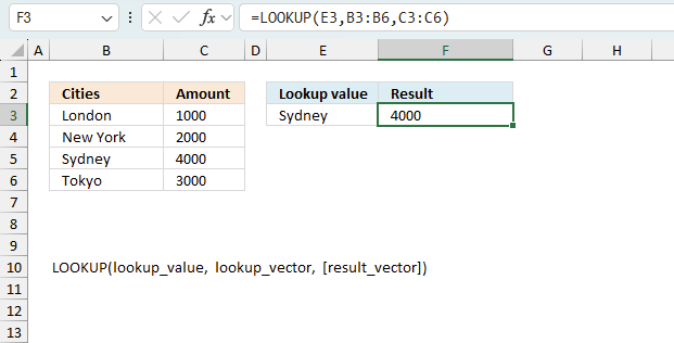
The LOOKUP function lets you find a value in a cell range and return a corresponding value on the same row. The lookup_vector must be sorted in ascending order for this function to work properly. Ascending order means that the values are sorted from A to Z or small to large if numerical. I recommend using the newer XLOOKUP function or the VLOOKUP function if the XLOOKUP function is not available in your Excel version.
Table of Contents
- Syntax
- Be careful
- Find the largest value in lookup_vector that is less than or equal to lookup_value
- How to use multiple values
- Multiple worksheets
- Nested LOOKUP functions
- How to lookup multiple values simultaneously (array formula)
- Get Excel file
- Find last matching value in an unsorted list
- Lookup and match last value - reverse lookup
- Function not working
1. Syntax
LOOKUP(lookup_value, lookup_vector, [result_vector])
If the LOOKUP function can't find the lookup_value, the function matches the largest value in lookup_vector that is less than or equal to lookup_value.
If lookup_value is smaller than the smallest value in lookup_vector, LOOKUP returns the #N/A error value.
| lookup_value | Required. The lookup value can be a number, text or a logical value. It can also be a cell reference. This argument can also handle multiple values but you need to enter it as an array function to make it work, there is an example later in this post. |
| lookup_vector | Required. This argument must be a single column or single row cell range. |
| result_vector | Required. The result vector is optional. If omitted the function returns the lookup value, if found. This argument must be a single column or single row cell range and have the same size as the lookup vector. |
3. Be careful with the LOOKUP function
The values in lookup_vector must be sorted ascending or from A to Z but that is not all. You may think you get an error if the lookup value is not found but that is not always the case.
Only if the lookup_value is smaller than the smallest value in lookup_vector, LOOKUP returns #N/A. See cell B4 and C4 in this animated picture.
So why does "Rome" return 2000? LOOKUP function can't find the lookup_value so it matches the largest value in lookup_vector that is less than or equal to lookup_value.
If Rome would have been in this sorted list, it would be between New York and Sydney. New York is less (alphabetically) than Rome but greater than London. The corresponding value to New York is returned, that value is 2000.
Anchorage is smaller than the smallest value "London" (alphabetically) and Lookup returns #N/A.
You really need to know what you are doing if you are going to use this function. I do recommend using this function with numerical ranges, see next example.
4. Find the largest value in lookup_vector that is less than or equal to lookup_value

This example uses a numerical value as a lookup value specified in cell B3. If an exact match is not found the closest value is returned as long as it is smaller than the lookup value.
Formula in cell C3:
becomes
LOOKUP(1.15, {1.03,1.09,1.16,1.22,1.29}, {"A","B","C","D","E"})
and returns "B" in cell C3..
The largest value that is smaller or equal to 1.15 is 1.09. The corresponding value to 1.09 is B.
5. How to use multiple values in the LOOKUP function

You can concatenate values and search two columns, use the ampersand character "&" to concatenate values in an argument.
Note that the table is sorted by column B and then by column C. This is required in order to get reliable results.
Formula in cell D3:
Explaining formula in cell D2
LOOKUP(lookup_value, lookup_vector, [result_vector])
Step 1 - Concatenate lookup_value
B3&C3
becomes
2012&"A"
and returns "2012A".
Step 2 - Concatenate lookup_vector
B7:B12&C7:C12
becomes
{2011; 2011; 2011; 2012; 2012; 2012}&{"A"; "B"; "C"; "A"; "B"; "C"}
and returns
{"2011A"; "2011B"; "2011C"; "2012A"; "2012B"; "2012C"}
Step 3 - Evaluate LOOKUP function
LOOKUP(B3&C3, B7:B12&C7:C12, D7:D12)
becomes
LOOKUP("2012A", {"2011A"; "2011B"; "2011C"; "2012A"; "2012B"; "2012C"}, {10;20;30;40;50;60})
and returns 40 in cell D3.
6. How to make the LOOKUP function work with multiple worksheets

This formula allows you to specify a sheet name and a lookup value. The INDIRECT function returns the cell reference depending on the value in cell B3.
Formula in cell D3:
Explaining formula in cell D2
Note that the table is sorted by column B and then by column C. This is required in order to use the LOOKUP function.
LOOKUP(lookup_value, lookup_vector, [result_vector])
Step 1 - Create cell reference to another worksheet (lookup_vector)
The INDIRECT function is able to create a working cell reference containing a worksheet name specified in cell B3.
Change the worksheet name and the LOOKUP function changes immediately to the given worksheet name.
INDIRECT(B3&"!B6:B8")
becomes
INDIRECT("2000!B6:B8")
and returns "2000!B6:B8". Note that there is an exclamation mark between the worksheet name and the cell reference.
Step 2 - Create cell reference to another worksheet ([result_vector])
INDIRECT(B3&"!C6:C8")
becomes
INDIRECT("2000!C6:C8")
and returns "2000!C6:C8".
Step 3 - Evaluate LOOKUP function
LOOKUP(C3,INDIRECT(B3&"!B6:B8"),INDIRECT(B3&"!C6:C8"))
becomes
LOOKUP("B", 2000!B6:B8, 2000!C6:C8)
becomes
LOOKUP("B", {"A"; "B"; "C"}, {1.1; 1.2; 1.3})
and returns 1.2 in cell D3.
7. Nested LOOKUP functions
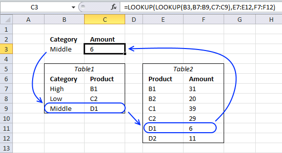
This formula looks for a value in table1 and uses the corresponding value to do another lookup in table2. The tables must be related meaning they share at least one column with the same values, in this case column "Product".
Formula in cell C3:
You can see that the Product column exists in both these tables, the tables are related.
Explaining formula in cell C3
Note that Table1 is sorted by column B and then by column C, both columns from A to Z.
This is true for Table2 as well, it is sorted by column E and then by column F from A to z.
Step 1 - Find value in B7:B9 and return the corresponding value from C7:C9
LOOKUP(B3, B7:B9, C7:C9)
becomes
LOOKUP("Middle", {"High"; "Low"; "Middle"}, {"B1"; "C2"; "D1"})
and returns "D1".
Step 2 - Evaluate the second LOOKUP function
LOOKUP(LOOKUP(B3, B7:B9, C7:C9), E7:E12, F7:F12)
becomes
LOOKUP("D1", E7:E12, F7:F12)
becomes
LOOKUP("D1", {"B1"; "B2"; "C1"; "C2"; "D1"; "D2"}, {31; 20; 39; 29; 6; 11})
and returns 6 in cell C3.
I have made more formulas for related tables, see these posts:
- Search for values in a related table
- Sum values in a related table
- Extract unique distinct values from a related table
- Working with three related tables
- Applying conditional formatting to related tables
8. How to lookup multiple values simultaneously (array formula)
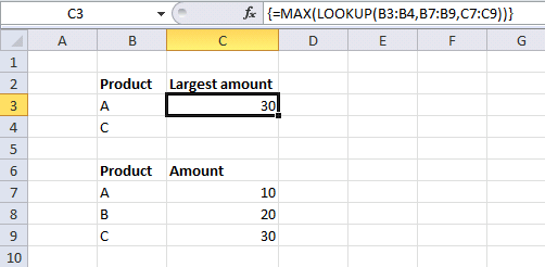
The first argument lookup_value allows you to enter not only a single value but multiple values. The LOOKUP function returns an array that has the same size as the lookup_value, to demonstrate this I made this formula:
Array formula in cell C3:
Note that it is required to enter the formula as an array formula if you have an earlier Excel version than Excel 365.
How to enter an array formula

- Select a cell.
- Copy/Paste the formula to the cell.
- Press and hold CTRL + SHIFT simultaneously.
- Press Enter once.
- Release all keys.
If you did this right the formula begins with a curly bracket { and ends with a curly bracket }. See the formula bar in the picture above.
These characters appear automatically, don't enter these chars yourself.
Explaining formula in cell C3
Note that the columns must be sorted from A to Z or smallest to largest.
Step 1 - Evaluate LOOKUP function
LOOKUP(B3:B4,B7:B9,C7:C9)
becomes LOOKUP({"A";"C"},{"A";"B";"C"},{10;20;30})
and returns this array {10;30}.
Step 2 - Extract maximum value from array
The MAX function returns the largest value from a cell range or array.
MAX(LOOKUP(B3:B4,B7:B9,C7:C9))
becomes
MAX({10;30})
and returns 30 in cell C3.
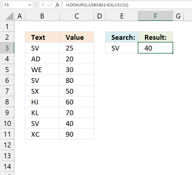
10. Find last matching value in an unsorted list

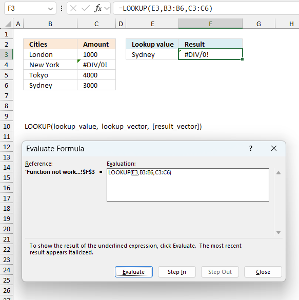
This article demonstrates a formula that returns the last matching value based on a given condition. The above image shows the lookup value in cell E3 and the formula in cell F3.
The formula uses the condition in cell E3 to find the last matching value in cell range B3:B11 and returns the corresponding value on the same orw from cell range F3:F11.
I read an interesting blog post Find Last Item in Group With Index Match written by Debra Dalgleish. It is about finding the last matching value in a sorted list. It got me thinking how to find the last matching item in an unsorted list.
This picture shows random text strings in column B and values in column C. Cell E3 contains the search value and F3 contains an array formula that returns the last matching value in a list.

Formula in cell F3:
This formula is a regular formula if you are an Excel 365 subscriber, however, if you use an earlier Excel version you need to enter the formula as an array formula.
How to enter an array formula
- Copy the above formula.
- Double press with left mouse button on with the left mouse button on cell F3.
- Paste formula to cell.
- Press and hold CTRL + SHIFT simultaneously.
- Press Enter once.
- Release all keys.
Learn to add more criteria:
Recommended articles
This article shows a formula that performs a reverse lookup and returns the corresponding value based on the last matching […]
10.1 Explaining the formula in cell F3

The Evaluate Formula tool lets you see formula calculations in greater detail. Press with left mouse button on with left mouse button on cell F3 to select it. Go to the "Formula" tab on the ribbon. Press with left mouse button on the "Evaluate Formula" button and a dialog box appears, see above image.
You can now examine and troubleshoot the formula using the "Evaluate" button on the dialog box. It will, step by step, go through the calculation. The underlined expression is what is about to be evaluated and the italicized expression is the result of the most recent evaluation.
Keep press with left mouse button oning the "Evaluate" button to see all calculations. You will see the final result when all calculations are made, that value will match the value returned in cell F3. The "Close" button dismisses the dialog box when you are done evaluating.
Step 1 - Find matching values
The logical operators allow you to create a logical expression, they are : = < > and can also be combined.
= equal
> larger than
< smaller than
<> not equal to
=> larger than or equal to
=< smaller than or equal to
A logical expression returns a boolean value TRUE or FALSE. Note, they have numerical equivalents. TRUE anything but zero and FALSE = 0 (zero).
The following logical expression returns an array corresponding to cell range B3:B11.
B3:B11=E3
becomes
{"SV"; "AD"; "WE"; "SV"; "SX"; "HJ"; "KL"; "SV"; "XC"}="SV"
Arrays has delimiting characters, a ; (semicolon) means that the values are in a column. A , (comma) separates values in a row. An array may contain values from a cell range containing multiple rows and columns, this means that the array contains both ; and , to indicate their positions in the cell range.
returns
{TRUE; FALSE; FALSE; TRUE; FALSE; FALSE; FALSE; TRUE; FALSE}
TRUE means that the value is equal to the value in cell E3.

Step 2 - Divide 1 with array
The LOOKUP function lets you find a value in a cell range and return a corresponding value on the same row, however, it also ignores error values and returns the last match which is surprising. I will show you how in step 3.
LOOKUP(lookup_value, lookup_vector, [result_vector])
The [result_vector] argument is optional. To create an error replacing the boolean value FALSE I simply divide 1 with the array.
1/(B3:B11=E3)
The parentheses allow you to control the order of operation meaning we want the formula to first calculate the logical expression and then divide 1 with the resulting array.
1/(B3:B11=E3)
becomes
1/{TRUE; FALSE; FALSE; TRUE; FALSE; FALSE; FALSE; TRUE; FALSE}
and returns
{1; #DIV/0!; #DIV/0!; 1; #DIV/0!; #DIV/0!; #DIV/0!; 1; #DIV/0!}
The #DIV/0! error is returned if you try to divide something with zero which is not possible.

The above image shows the array in cell range D3:D11, Excel shows a green triangle in the top left corner indicating that the value is an error value.
Step 3 - Find last value in array
The lookup_value must be larger than the values in the loop_vector and the values in the lookup_vector must be the same in order to get the last value that matches the lookup_value.
LOOKUP(lookup_value, lookup_vector, [result_vector])
LOOKUP(2,1/(B3:B11=E3),C3:C11)
becomes
LOOKUP(2,{1; #DIV/0!; #DIV/0!; 1; #DIV/0!; #DIV/0!; #DIV/0!; 1; #DIV/0!},{25; 20; 30; 80; 50; 60; 70; 40; 90})
Step 4 - Return corresponding value
LOOKUP(2,1/(B3:B11=E3),C3:C11)
returns 40 in cell F3.
The last value matching the condition has the relative position eight in the array, the corresponding value in cell range C3:C11 is 40.

10. Lookup and match last value - reverse lookup
This section shows a formula that performs a reverse lookup and returns the corresponding value based on the last matching value.
Table of Contents
- Lookup and match the last value
- Lookup and match last value - two conditions AND - logic
- Find the last matching value - two conditions OR - logic
- Find the last matching value based on a list of values
- Find the last matching date based on a date range
- Lookup week and match last value
- Lookup month and match last value
- Lookup year and match the last value
- How to perform a reverse lookup - Excel 365 (Link)
- Get *.xlsx file
10.1. Find the last matching value
The formula in cell F3 performs a lookup and matches the last item, it returns a corresponding value from column C on the same row.
For example, Item "SV" is found in cells B3, B6, and B10. The last matching value is in cell B10 and the corresponding value in column C is "40".
Formula in cell F3:
I recommend the XLOOKUP function if you use Excel 365.
10.1.1 Explaining formula in cell F3
Step 1 - Compare values to search value
The equal sign compares value to value, you can also compare a single value to multiple values at the same time. That is what is going on here.
B3:B11=E3
returns {TRUE; FALSE; ... ; FALSE}.
Step 2 - Divide 1 with result
The parentheses let you control the order of calculations, we want to perform the comparison before the division with 1.
1/(B3:B11=E3)
returns {1; #DIV/0!; ... ; #DIV/0!}.
Step 3 - Lookup the last matching value
The LOOKUP function allows us to match a value if it is sorted ascending, however it also lets you match the last value in an array if the others are errors.
LOOKUP(2,1/(B3:B11=E3),C3:C11)
returns 40.
10.2. Find the last matching value - two conditions AND - logic
10.2.1 Question
Ok, you've shown it for regular ranges....how about within tables.I have a table similar to:ID Name Date
1001 Joe Smith 5/1/2017
1002 John Doe 5/2/2017
1001 Joe Smith 5/17/2017
1003 Jane Doe 5/18/2017
1001 Joe Smith 5/20/2017
10.2.2 Formula
The formula below lets you search for criteria and return the last matching record in the table.
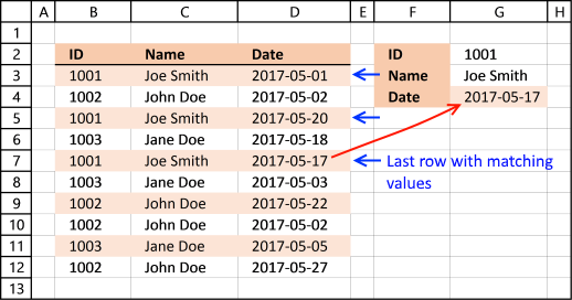
Example, 1001 and Joe Smith is found on row 3,5 and 7. The record on row 7 is the last record in the table so the formula returns the date (2017-05-17) from row 7, in cell G4.
Formula in cell G4:
This formula is weird, you don't need to enter it as an array formula as you should. I don't know why, however this gave me an idea, check it out here:
Create a list of unique distinct values
Recommended article
Recommended articles
This article demonstrates a formula that returns the last matching value based on a given condition. The above image shows […]
10.2.3 Explaining formula in cell G4
Step 1 - Construct first logical expression (ID)
We want to find all to find values in column B equal to 1001. The equal sign lets you compare value to values, not case sensitive.
B3:B12=G2
returns {TRUE; FALSE; ... ; FALSE}
Step 2 - Construct second logical expression (NAME)
The second logical expressions checks if values in cell range C3:C12 is equal to "Joe Smith"
C3:C12=G3
returns {TRUE; FALSE; ... ; FALSE}
Step 3 - Multiply arrays
Both conditions must be met so we must multiply (*) the arrays. If we wanted at least one of two conditions met we would add the arrays (+)
(B3:B12=G2)*(C3:C12=G3)
returns {1; 0; 1; 0; 1; 0; 0; 0; 0; 0}
Step 4 - Dividing by zero returns an error
The LOOKUP function allows us to match a value if it is sorted ascending, however it also lets you match the last value in an array if the others are errors.
1/((B3:B12=G2)*(C3:C12=G3))
and returns
{1;#DIV/0!;1;#DIV/0!; 1;#DIV/0!; #DIV/0!; #DIV/0!;#DIV/0!; #DIV/0!}
1/0 returns #DIV/0!
Step 5 - Find the last value in the array
The LOOKUP function finds the last value in the array and returns the corresponding value on the same row in cell range D3:D12.
LOOKUP(2,1/((B3:B12=G2)*(C3:C12=G3)),D3:D12)
returns 2017-05-17 (42872) in cell G4.
Recommended articles
Finds a value in a sorted cell range and returns a value on the same row.
10.3. Find the last matching value - two conditions OR - logic

The image above demonstrates a formula in cell G4 that returns a value if at least one of two possible conditions match on the same row, however, the formula performs a reverse lookup meaning it starts with the last value and moves up. As soon as any of the two conditions match the corresponding value from column D is returned.
For example, the first condition is specified in cell G2 and the second is specified in cell G3. The formula starts with the last row (12) and goes up. "Jane Doe" is the first match in cell C11, the formula returns the corresponding value "5/5/2017" from column D on the same row (11).
Formula in cell G4:
10.3.1 Explaining formula in cell G4
Step 1 - Compare first lookup value to values
The equal sign is a logical operator meaning it lets you compare value to values, not case sensitive. The result is a logical value or boolean value, in this case, multiple values.
B3:B12=G2
returns {TRUE; ... ; FALSE}.
Step 2 - Compare second lookup value to values
C3:C12=G3
returns {FALSE; ... ; FALSE}.
Step 3 - Add array values
The plus sign adds the arrays containing boolean values.
(B3:B12=G2)+(C3:C12=G3)
returns {1; 0; 1; 1; 1; 1; 0; 0; 1; 0}.
Step 4 - Divide 1 with array
We want to create an error value if the array contains a 0 (zero). The LOOKUP function ignores error values.
1/((B3:B12=G2)+(C3:C12=G3))
returns {1; #DIV/0!; 1; 1; 1; 1; #DIV/0!; #DIV/0!; 1; #DIV/0!}.
Step 5 - Find a match and return the corresponding value
The LOOKUP function allows us to match a value if it is sorted ascending, however it also lets you match the last value in an array if the others are errors.
LOOKUP(2, 1/((B3:B12=G2)+(C3:C12=G3)), D3:D12)
returns 42860 (5/5/2017).
10.4. Find the last matching value based on a list of values

The formula in cell G3 shown in the image above performs a reverse lookup using multiple values specified in cell range E3:E5. It starts with the last value which is cell B11 and checks if any of the values match.
The last lookup value "XC" matches cell B11 so the formula returns the corresponding value from column C on the same row which is "90".
Formula in cell G3:
10.4.1 Explaining formula in cell G3
Step 1 - Count values based on list
The COUNTIF function counts values matching any value in cell range E3:E5.
COUNTIF(E3:E5, B3:B11)
returns {1; 1; 0; 1; 0; 0; 0; 1; 1}.
Step 2 - Divide 1 with array
We want to create an error value if the array contains a 0 (zero). The LOOKUP function ignores error values which will be demonstrated in the next step.
1/COUNTIF(E3:E5, B3:B11)
returns {1; 1; #DIV/0!; 1; #DIV/0!; #DIV/0!; #DIV/0!; 1; 1}.
Step 3 - Lookup value and return corresponding value
The LOOKUP function allows you to match the last value in an array (reverse lookup) if the other values are errors.
LOOKUP(2, 1/COUNTIF(E3:E5, B3:B11), C3:C11)
becomes
LOOKUP(2, {1; 1; #DIV/0!; 1; #DIV/0!; #DIV/0!; #DIV/0!; 1; 1}, {25; 20; 30; 80; 50; 60; 70; 40; 90})
and returns 90 in cell G3.
10.5. Find the last matching date based on a date range

The image above demonstrates a formula in cell F4 that uses a date range specified in cell F2 and F3 to perform a reverse lookup using all dates in the date range against dates in cell range B3:B12.
For example, the formula begins with the last date which is in cell B12, and moves up. There is not a match until cell B10 which contains the date "5/2/2017", that date is in the date range specified in cells F2:F3.
The corresponding value from the same row in column C is "1002", that value is returned in cell F4.
Formula in cell F4:
10.5.1 Explaining formula in cell F4
Step 1 - Compare end date to dates
The less than and equal sign combined checks if the dates are equal or smaller than the end date.
C3:C12<=G3
returns {TRUE; ... ; FALSE}.
Step 2 - Compare start date to dates
The larger than and equal sign combined checks if the dates are equal or larger than the start date.
C3:C12>=G2
returns {FALSE; TRUE; ... ; TRUE}.
Step 3 - Multiply arrays
The asterisk character lets you multiply the arrays meaning you apply AND logic. AND logic works like this: TRUE*TRUE = TRUE (1) , TRUE * FALSE = FALSE (0)
When you perform a calculation in Excel boolean values are converted to their numerical equivalents. TRUE = 1 and FALSE = 0 (zero)
(C3:C12<=G3)*(C3:C12>=G2)
returns {0; 1; 0; 0; 0; 1; 0; 1; 0; 0}.
Step 4 - Divide 1 with array
1/((C3:C12<=G3)*(C3:C12>=G2))
returns {#DIV/0!; 1; ... ; #DIV/0!}.
Step 5 - Reverse lookup based on date range
LOOKUP(2, 1/((C3:C12<=G3)*(C3:C12>=G2)), D3:D12)
returns 1002.
10.6. Find the last matching week

The image above shows a formula in cell G3 that performs a reverse lookup using a week number specified in cell G2.
It returns a value from column D if the corresponding cell in column C matches the lookup value.
Formula in cell G3:
10.6.1 Explaining formula in cell G3
Step 1 - Convert dates to week numbers
The ISOWEEKNUM function calculates a number based on the ISO week number of the year for a given date.
ISOWEEKNUM(C3:C12)
returns {18; 18; 20; 20; 20; 18; 21; 18; 18; 21}.
Step 2 - Compare week numbers to the condition
ISOWEEKNUM(C3:C12)=G2
returns {TRUE; TRUE; FALSE; FALSE; FALSE; TRUE; FALSE; TRUE; TRUE; FALSE}.
Step 3 - Divide 1 with array
1/(ISOWEEKNUM(C3:C12)=G2)
returns {1; 1; #DIV/0!; #DIV/0!; #DIV/0!; 1; #DIV/0!; 1; 1; #DIV/0!}.
Step 4 - Reverse lookup based on week number
LOOKUP(2, 1/(ISOWEEKNUM(C3:C12)=G2), D3:D12)
returns 1003.
10.7. Find the last matching month

The picture above demonstrates a formula in cell G3 that performs a reverse lookup using a month number specified in cell G2.
It returns a value from column D if the corresponding cell in column C matches the lookup value.
For example, column B contains numbers representing the relative position of a month. 1 is January, 2 is February ... 12 is December.
Cell G2 contains 4, the formula starts with the last cell in column C and goes up. Cell C10 contains a date in April which is month number 4, it matches number 4 in cell G2.
The corresponding value in column D on the same row is returned to cell G3.
Formula in cell G3:
10.7.1 Explaining formula in cell G3
Step 1 - Calculate number representing the month
The MONTH function calculates the month as a number from an Excel date.
MONTH(C3:C12)
returns {5; 4; 5; 5; 5; 5; 5; 4; 5; 5}.
Step 2 - Compare month numbers to lookup value
MONTH(C3:C12)=G2
returns {FALSE; TRUE; FALSE; FALSE; FALSE; FALSE; FALSE; TRUE; FALSE; FALSE}.
Step 3 - Divide 1 with array
1/(MONTH(C3:C12)=G2)
returns {#DIV/0!; 1;... ; #DIV/0!}.
Step 4 - Reverse lookup based on month number
LOOKUP(2, 1/(MONTH(C3:C12)=G2), D3:D12)
returns 1002.
10.8. Find the last matching year

The formula in cell G3 performs a reverse lookup using the year number in cell G2 against dates in column C.
The last match is found in cell C11 and the corresponding value in column D on the same row is returned to cell G3.
Formula in cell G3:
10.8.1 Explaining formula in cell G3
Step 1 - Calculate year
The YEAR function extracts the year from an Excel date.
YEAR(C3:C12)
returns {2017; 2018; 2019; ... ; 2017}.
Step 2 - Compare year numbers to lookup value
YEAR(C3:C12)=G2
returns {FALSE; ... ; FALSE}
Step 3 - Divide 1 with array
1/(YEAR(C3:C12)=G2)
returns {#DIV/0!; 1; ... ; #DIV/0!}.
Step 4 - Lookup year and return value based on last match
LOOKUP(2, 1/(YEAR(C3:C12)=G2), D3:D12)
returns 1003 in cell G3.
11. Function not working
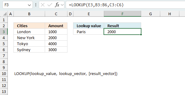
The image above shows what happens if the lookup_value is not found. The function returns 2000 which corresponds to "New York", "Paris" is between "New York" and "Tokyo" if sorted from A to Z.
The LOOKUP function returns
- #NAME? error if you misspell the function name.
- propagates errors, meaning that if the input contains an error (e.g., #VALUE!, #REF!), the function will return the same error.
11.1 Troubleshooting the error value
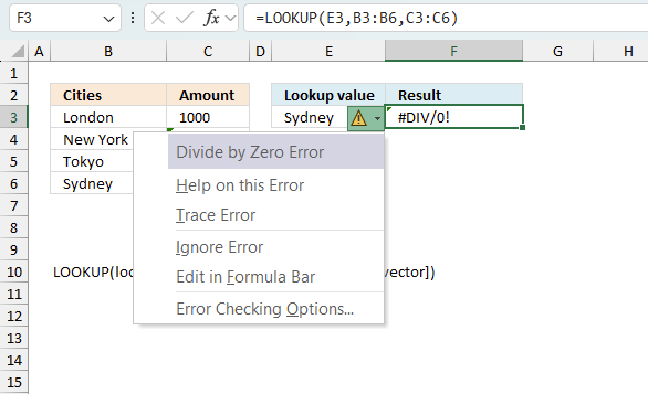
When you encounter an error value in a cell a warning symbol appears, displayed in the image above. Press with mouse on it to see a pop-up menu that lets you get more information about the error.
- The first line describes the error if you press with left mouse button on it.
- The second line opens a pane that explains the error in greater detail.
- The third line takes you to the "Evaluate Formula" tool, a dialog box appears allowing you to examine the formula in greater detail.
- This line lets you ignore the error value meaning the warning icon disappears, however, the error is still in the cell.
- The fifth line lets you edit the formula in the Formula bar.
- The sixth line opens the Excel settings so you can adjust the Error Checking Options.
Here are a few of the most common Excel errors you may encounter.
#NULL error - This error occurs most often if you by mistake use a space character in a formula where it shouldn't be. Excel interprets a space character as an intersection operator. If the ranges don't intersect an #NULL error is returned. The #NULL! error occurs when a formula attempts to calculate the intersection of two ranges that do not actually intersect. This can happen when the wrong range operator is used in the formula, or when the intersection operator (represented by a space character) is used between two ranges that do not overlap. To fix this error double check that the ranges referenced in the formula that use the intersection operator actually have cells in common.
#SPILL error - The #SPILL! error occurs only in version Excel 365 and is caused by a dynamic array being to large, meaning there are cells below and/or to the right that are not empty. This prevents the dynamic array formula expanding into new empty cells.
#DIV/0 error - This error happens if you try to divide a number by 0 (zero) or a value that equates to zero which is not possible mathematically.
#VALUE error - The #VALUE error occurs when a formula has a value that is of the wrong data type. Such as text where a number is expected or when dates are evaluated as text.
#REF error - The #REF error happens when a cell reference is invalid. This can happen if a cell is deleted that is referenced by a formula.
#NAME error - The #NAME error happens if you misspelled a function or a named range.
#NUM error - The #NUM error shows up when you try to use invalid numeric values in formulas, like square root of a negative number.
#N/A error - The #N/A error happens when a value is not available for a formula or found in a given cell range, for example in the VLOOKUP or MATCH functions.
#GETTING_DATA error - The #GETTING_DATA error shows while external sources are loading, this can indicate a delay in fetching the data or that the external source is unavailable right now.
11.2 The formula returns an unexpected value
To understand why a formula returns an unexpected value we need to examine the calculations steps in detail. Luckily, Excel has a tool that is really handy in these situations. Here is how to troubleshoot a formula:
- Select the cell containing the formula you want to examine in detail.
- Go to tab “Formulas” on the ribbon.
- Press with left mouse button on "Evaluate Formula" button. A dialog box appears.
The formula appears in a white field inside the dialog box. Underlined expressions are calculations being processed in the next step. The italicized expression is the most recent result. The buttons at the bottom of the dialog box allows you to evaluate the formula in smaller calculations which you control. - Press with left mouse button on the "Evaluate" button located at the bottom of the dialog box to process the underlined expression.
- Repeat pressing the "Evaluate" button until you have seen all calculations step by step. This allows you to examine the formula in greater detail and hopefully find the culprit.
- Press "Close" button to dismiss the dialog box.
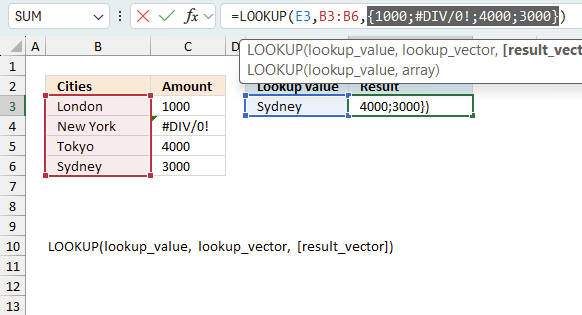
There is also another way to debug formulas using the function key F9. F9 is especially useful if you have a feeling that a specific part of the formula is the issue, this makes it faster than the "Evaluate Formula" tool since you don't need to go through all calculations to find the issue.
- Enter Edit mode: Double-press with left mouse button on the cell or press F2 to enter Edit mode for the formula.
- Select part of the formula: Highlight the specific part of the formula you want to evaluate. You can select and evaluate any part of the formula that could work as a standalone formula.
- Press F9: This will calculate and display the result of just that selected portion.
- Evaluate step-by-step: You can select and evaluate different parts of the formula to see intermediate results.
- Check for errors: This allows you to pinpoint which part of a complex formula may be causing an error.
The image above shows cell reference C3:C6 converted to hard-coded value using the F9 key. The LOOKUP function requires non-error values which is not the case in this example. We have found what is wrong with the formula.
Tips!
- View actual values: Selecting a cell reference and pressing F9 will show the actual values in those cells.
- Exit safely: Press Esc to exit Edit mode without changing the formula. Don't press Enter, as that would replace the formula part with the calculated value.
- Full recalculation: Pressing F9 outside of Edit mode will recalculate all formulas in the workbook.
Remember to be careful not to accidentally overwrite parts of your formula when using F9. Always exit with Esc rather than Enter to preserve the original formula. However, if you make a mistake overwriting the formula it is not the end of the world. You can “undo” the action by pressing keyboard shortcut keys CTRL + z or pressing the “Undo” button
11.3 Other errors
Floating-point arithmetic may give inaccurate results in Excel - Article
Floating-point errors are usually very small, often beyond the 15th decimal place, and in most cases don't affect calculations significantly.
'LOOKUP' function examples

First, let me explain the difference between unique values and unique distinct values, it is important you know the difference […]
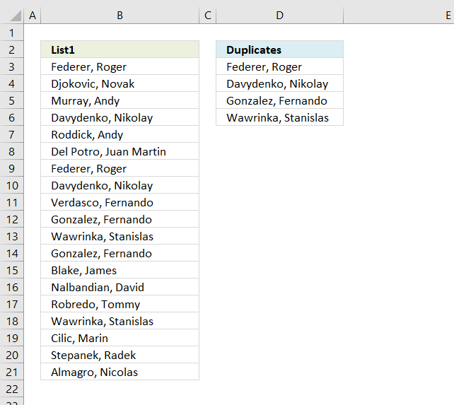
The array formula in cell C2 extracts duplicate values from column A. Only one duplicate of each value is displayed […]
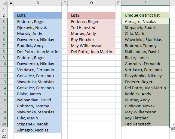
Question: I have two ranges or lists (List1 and List2) from where I would like to extract a unique distinct […]
Functions in 'Lookup and reference' category
The LOOKUP function function is one of 25 functions in the 'Lookup and reference' category.
Excel function categories
Excel categories
24 Responses to “How to use the LOOKUP function”
Leave a Reply
How to comment
How to add a formula to your comment
<code>Insert your formula here.</code>
Convert less than and larger than signs
Use html character entities instead of less than and larger than signs.
< becomes < and > becomes >
How to add VBA code to your comment
[vb 1="vbnet" language=","]
Put your VBA code here.
[/vb]
How to add a picture to your comment:
Upload picture to postimage.org or imgur
Paste image link to your comment.
=INDEX(C2:C11,MAX(IF(B2:B11=E3,ROW(B2:B11)-1)))
sam,
I try to make formulas that work in any cell without any user interaction. That is why my formulas are sometimes a bit longer.
Thanks for commenting!
If you have Excel 2010> use the INDEX & AGGREGATE for a non array formula.
=INDEX(C3:C11,AGGREGATE(14,6,ROW(B3:B11)-ROW(B2)/(B3:B11=E3),1))
Kevin,
Interesting formula, thank you for commenting.
Sam,
your formula is not robust. If any row inserted above the table it will produce inaccurate value.
Oscar,
my array version is
=INDEX($C$3:$C$11,MATCH(1,--($E$3=$B$3:$B$11),1))
or, for those who is afraid of array formula,
=INDEX($C$3:$C$11,MATCH(1,INDEX(--($E$3=$B$3:$B$11),),1))
I like the idiom MATCH(ROW($B$3:$B$11),ROW($B$3:$B$11)) you used to generate a numeric sequence, but ROW($B$3:$B$11)-ROW($B$2) should be quicker.
Leonid,
I can´t get your formula working. If I change the value in cell B10 this happens, see picture:
Good catch. This slight modification should fix the problem:
array
=INDEX(C3:C11,MATCH(1,1/(E3=B3:B11),1))
non array
=INDEX(C3:C11,MATCH(1,INDEX(1/(E3=B3:B11),),1))
Leonid,
Thank you for your solution.
I don´t understand why this works
MATCH(1, {1; #DIV/0!; #DIV/0!; 1; #DIV/0!; #DIV/0!; #DIV/0!; #DIV/0!; #DIV/0!}, 1)
but this does not
MATCH(1,{1;0;0;1;0;0;0;0;0},1)
[…] Recently, I shared a formula for finding the last item in a category, in a sorted list. Oscar created a formula that works with an unsorted list. […]
Hi
=LOOKUP(2,1/($B$3:$B$11=E3),$C$3:$C$11)
Xlarium..Thanks! Works perfectly!
Is there a way to specify which kth largest/smallest value to return?
Thanks for this. Very useful. Only thing is that it returns a result (10) even if the search value does not appear in the list. Any thoughts?
Hello,
I only comment to say thaaank you so much!!. Very useful.
Only one thing. You should advertise that we have to press CONTROL+SHIFT+ENTER, instead of ONLY ENTER, to add the matriz formula.
How to do the same with double criteria.
Month Text Value
1 SV 10
1 AD 20
1 kl 30
1 SV 40
2 SX 50
2 HJ 60
2 KL 150
3 SV 80
3 XC 90
3 SV 50
3 ab 90
3 SV 70
I need below result.
Month Text Value:
3 sv 70
OR 2 KL 150
hi
See solution below
=INDEX(D1:D12,(MAX((C1:C12="sv")*(B1:B12=3)*ROW(C1:C12))))
Where Column B= Months Column C= Text and Column D = Values
I have a similar problem,
Im trying to make an excel where column A is a drop down box and the first 30 odd rows Column F finds a value from a different page i done this with VLookup all works find but now when i type in 'SV on column A i want column F to find the last value from SV on the same page, but there will be no orders to it- i am trying to do a stock take page when i order something in it gets added to stock if i ship something out it gets taken away from the value in column F
how can I use this formula with multiple criteria? I've already managed to do the simple one but I would like to find the last value of something by month.
Ok, you've shown it for regular ranges....how about within tables.
I have a table similar to:
ID Name Date
1001 Joe Smith 5/1/2017
1002 John Doe 5/2/2017
1001 Joe Smith 5/17/2017
1003 Jane Doe 5/18/2017
1001 Joe Smith 5/20/2017
DonW,
Check this out:
https://www.get-digital-help.com/find-last-matching-value-in-an-unsorted-table/
I need a way to find the last non empty value on an entry based on month columns.
https://imgur.com/a/Sf5YvUI
So as per above Image,
I had used =LOOKUP(2,1/($A:$A=$D$3),$B:$B) this formula to get value for month but for Jan it showing correct but for Month Feb it showing Value 0 instead of ABS-143-002 because last value for Month Feb empty cell.
I tried too much but not getting perfect answer for this
Please, help me with this I need non empty last value from column B for selected month without using VBA.
Gopi Sahane,
try this formula:
=LOOKUP(2,1/(($A1:$A1000=$D$3)*($B1:$B1000<>"")),$B1:$B1000)