Compare two columns and extract differences

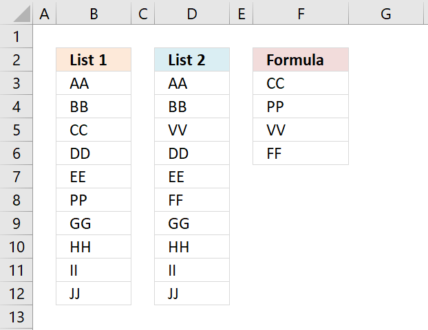
This article demonstrates formulas that extract values that exist only in one column out of two columns. There are text values in column B and column C displayed in the image above. Column E contains values that exist only in column B and column F contains values that exist only in column C.
The following posts describe how to extract rows or records by comparing two data sets:
This article demonstrates how to use conditional formatting to highlight differences and shared values:
How to highlight differences and common values in lists
Table of Contents
1. Introduction
Why compare values in two different columns?
Comparing values in two different columns in Excel is useful in many situations, such as:
- Finding Missing Data – When managing datasets like customer lists or inventory records. You can compare two columns to identify missing entries. For example, customers who purchased last year but not this year.
- Data De-duplication – Helps find duplicate or unique values when merging datasets such as checking for repeated email addresses in a contact list.
- Reconciling Financial Data – Ensures accuracy by comparing two financial reports such as identifying transactions recorded in one account but missing in another.
- Tracking Changes Over Time – Compares past and current data to detect changes such as employees who were on last month’s payroll but not this month’s.
- Validating Data Consistency – Ensures data integrity by checking if values in two columns match such as verifying product codes between two databases.
2. Compare two columns and extract differences - Excel 365

The formula in cell E3 extracts values in cell range B3:B15 that are not in cell range C3:C11, meaning they exist only in cell range B3:B15.
For example, value "AA" in cell B3 is not in cell range C3:C11, however, value "DD" in cell B5 is also in cell range C3:C11, in cell C4.
Excel 365 formula in cell E3:
The formula in cell F3 extracts values in cell range C3:C11 that are not in cell range B3:B15
Excel 365 formula in cell F3:
The dynamic Excel 365 formulas above are entered like regular formulas.
2.1 Explaining formula
Step 1 - Compare/Count values between C3:C11 and B3:B15
The COUNTIF function calculates the number of cells that is equal to a condition.
Function syntax: COUNTIF(range, criteria)
COUNTIF(C3:C11, B3:B15)
returns {0; 0; 1; 1; 0; 1; 1; 1; 1; 0; 0; 0; 1}.
Step 2 - Check if a number is equal to zero
The equal sign lets you compare value to value, it is also possible to compare multiple values to a value. The equal sign is a logical operator and returns a boolean value TRUE or FALSE.
COUNTIF(C3:C11,B3:B15)=0
becomes
{0; 0; 1; 1; 0; 1; 1; 1; 1; 0; 0; 0; 1}=0
and returns
{TRUE; TRUE; ... ; FALSE}.
Step 3 - Filter values based on boolean values
The FILTER function extracts values/rows based on a condition or criteria.
Function syntax: FILTER(array, include, [if_empty])
FILTER(B3:B15, COUNTIF(C3:C11, B3:B15)=0)
returns {"AA";"CC";"GG";"MM";"NN";"OO"}.
3. Compare two columns and extract differences - earlier versions
Array formulas for older Excel versions
The array formula in cell E3 extracts values existing only in column B, compared to column C:
The array formula in cell F3 extracts values existing only in column C, compared to column B:
How to enter array formula in cell E3:

- Copy above array formula (Ctrl + c).
- Select cell E3.
- Press with left mouse button on in the formula bar.
- Paste array formula (Ctrl + v) to the formula bar.
- Press and hold CTRL + SHIFT simultaneously.
- Press Enter once.
- Release all keys.
The formula is now an array formula. See the curly brackets, they tell you it is an array formula. Don't enter the curly brackets yourself, they appear if you enter it correctly, like this:
3.1 How to copy array formula

- Select cell E3.
- Copy (Ctrl + c).
- Select cell range E4:E8.
- Paste (Ctrl + v).
3.2 Explaining array formula in cell E3

I recommend the "Evaluate Formula" tool when you want to understand, troubleshoot or examine a specific formula.
Select the cell containing the formula you want to evaluate. Go to tab "Formulas" on the ribbon, press with left mouse button on the "Evaluate Formula" button, see image above.

A dialog box appears, it shows the formula and the button "Evaluate" below the formula allows you to go through the formula calculations step by step.
Step 1 - Count values in column C based on values in column B

The COUNTIF function lets you count values based on a condition, however, it is also possible to use multiple conditions but then the function returns an array of values instead of a single value.
This is what makes the formula an array formula. Here are the arguments in the COUNTIF function:
COUNTIF(range, criteria)
COUNTIF($C$3:$C$11, $B$3:$B$15)
returns the following array of values:
{0; 0; 1; 1; 0; 1; 1; 1; 1; 0; 0; 0; 1}
The position of each value in the array is very important, they make it possible to identify and extract the values we want. The position of each value in the array corresponds to the value in column B, see image above.
A 0 (zero) means that the value in column B is not found in column C. 1 is that the value in column B is found once in column C.
Step 2 - Check if they are equal to 0 (zero)

The equal sign checks if the values are equal to 0 (zero) and returns the boolean values TRUE or FALSE.
COUNTIF($C$3:$C$11, $B$3:$B$15)=0
becomes
{0; 0; 1; 1; 0; 1; 1; 1; 1; 0; 0; 0; 1}=0
and returns
{TRUE; TRUE; ... ; FALSE}
Step 3 - If they are equal to zero, return the corresponding relative row number

The IF function allows you to return a specific value if the logical test is TRUE and another value if FALSE.
IF(logical_test, [value_if_true], [value_if_false])
IF(COUNTIF($C$3:$C$11, $B$3:$B$15)=0, MATCH(ROW($B$3:$B$15), ROW($B$3:$B$15)), "")
becomes
IF({TRUE; TRUE; FALSE; FALSE; TRUE; FALSE; FALSE; FALSE; FALSE; TRUE; TRUE; TRUE; FALSE}, MATCH(ROW($B$3:$B$15), ROW($B$3:$B$15)), "")
The MATCH and ROW functions create an array from 1 to 11 which we then will use to extract the correct value from cell range B3:B15.
MATCH(ROW($B$3:$B$15), ROW($B$3:$B$15))
returns {1; 2; ... ; 13}.
Step 4 - Return the k-th smallest row number
The SMALL function returns the k-th smallest number from an array or cell range.
SMALL(IF(COUNTIF($C$3:$C$11, $B$3:$B$15)=0, MATCH(ROW($B$3:$B$15), ROW($B$3:$B$15)), ""), ROWS($A$1:A1))
beomes
SMALL({1; 2; ... ; 13}, ROWS($A$1:A1))
The ROWS function counts the number of rows in a given cell reference. The cell ref in this example expands when you copy the cell and paste to cells below. This makes the SMALL function return a new number in each cell.
becomes
SMALL({1; 2; 3; 4; 5; 6; 7; 8; 9; 10; 11; 12; 13}, 1)
and returns 1.
Step 5 - Return value

The INDEX function returns a value or multiple values based on a row and/or column number.
INDEX($B$3:$B$15, SMALL(IF(COUNTIF($C$3:$C$11, $B$3:$B$15)=0, MATCH(ROW($B$3:$B$15), ROW($B$3:$B$15)), ""), ROWS($A$1:A1)))
becomes
INDEX($B$3:$B$15, 1)
and returns "AA" in cell E3.
4. How to extract not shared values in two columns
Question: How do I remove common values between two lists?
Answer: I created the formulas demonstrated in this section, they list the values from both columns List1 and List2 if they only exist in one or the other column, as seen on the picture above.
Excel 365 dynamic array formula in cell F3:
Excel 365 dynamic array formulas are entered as regular formulas.
Array formula in cell F3 for older Excel versions:
To enter an array formula, type the formula in cell B3 then press and hold CTRL + SHIFT simultaneously, now press Enter once. Release all keys.
 The formula bar now shows the formula with a beginning and ending curly bracket telling you that you entered the formula successfully.
Don't enter the curly brackets yourself, they appear automatically.
4.1 Explaining formula in cell F3
Step 1 - Count values
The COUNTIF function lets you count values based on a condition or criteria. COUNTIF(range, criteria) The first argument is the cell range you want to evaluate.
 The criteria argument contains the values you want to look for.
COUNTIF($D$3:$D$12,$B$3:$B$12)
becomes
COUNTIF({"AA"; "BB"; "VV"; "DD"; "EE"; "FF"; "GG"; "HH"; "II"; "JJ"},{"AA"; "BB"; "CC"; "DD"; "EE"; "PP"; "GG"; "HH"; "II"; "JJ"})
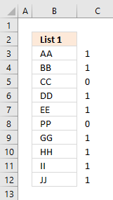
and returns the following array {1;1;0;1;1;0;1;1;1;1}.
The image to the right shows the array and the corresponding values, you can now easily see that CC and PP are not found in List 2.
Step 2 - Check if value is 0 (zero) and if so return the corresponding row number
If the array contains a zero the corresponding value is not found in the other list. The IF function lets you build a logical expression, if it evaluates to TRUE on thing happens and if FALSE another thing happens.
 IF(COUNTIF($D$3:$D$12, $B$3:$B$12)=0, MATCH(ROW($B$3:$B$12),ROW($B$3:$B$12)), "")
becomes
IF({1;1;0;1;1;0;1;1;1;1}, {1;2;3;4;5;6;7;8;9;10}, "")
and returns the following array:
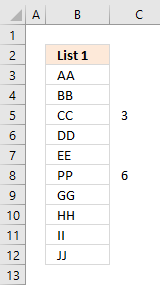
{"";"";3;"";"";6;"";"";"";""}
The image to the right shows the row numbers (relative to cell range $B$3:$B$12) in column C .
Step 3 - Extract the k-th smallest row number
The SMALL function returns the k-th smallest number from a cell range or an array. This allows us to extract a single value in a cell each.
SMALL(IF(COUNTIF($D$3:$D$12, $B$3:$B$12)=0, MATCH(ROW($B$3:$B$12),ROW($B$3:$B$12)), ""), ROWS($A$1:A1))
becomes
SMALL({"";"";3;"";"";6;"";"";"";""}, ROWS($A$1:A1))
becomes
SMALL({"";"";3;"";"";6;"";"";"";""}, 1)
and returns 3.
Step 4 - Get the corresponding value
The INDEX function returns a value based on a row and column number, the column number is not necessary if the cell range only has one column.
INDEX($B$3:$B$12, SMALL(IF(COUNTIF($D$3:$D$12, $B$3:$B$12)=0, MATCH(ROW($B$3:$B$12),ROW($B$3:$B$12)), ""), ROWS($A$1:A1)))
becomes
INDEX($B$3:$B$12, 3)
and returns the value in cell B5 which is "CC" to cell F3.
Step 5 - Return values from List 2
When there are no more values to extract from List 1 the IFERROR function lets you continue with List 2.
The formula is repeated in the second argument except that other cell ranges are used. I am not going to explain these steps again, see above steps if you need to.
The fomula in cell F5 becomes
IFERROR(INDEX($B$3:$B$12, SMALL(IF(COUNTIF($D$3:$D$12, $B$3:$B$12)=0,ROW($B$3:$B$12)-MIN(ROW($B$3:$B$12))+1,""),ROW(B1))),INDEX($D$3:$D$12, SMALL(IF(COUNTIF($B$3:$B$12,$D$3:$D$12)=0, ROW($D$3:$D$12)-MIN(ROW($D$3:$D$12))+1, ""), ROW(B1)-SUM((COUNTIF($D$3:$D$12,$B$3:$B$12)=0)+0))))
returns "VV" in cell F5.
Get Excel *.xlsx file
remove-common-values-between-two-columns4.xlsx
To create a unique list from two columns or two cell ranges, check this article out: Create unique list from two columns
Compare category
This article describes an array formula that compares values from two different columns in two worksheets twice and returns a […]
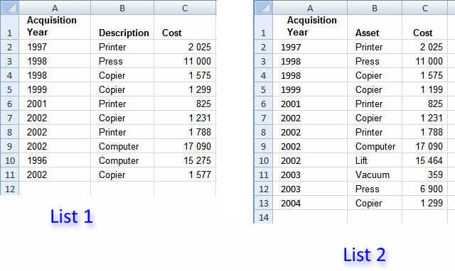
Table of Contents Compare tables: Filter records occurring only in one table Compare two lists and filter unique values where […]
This article demonstrates techniques to highlight differences and common values across lists. What's on this page How to highlight differences […]
Excel categories
6 Responses to “Compare two columns and extract differences”
Leave a Reply
How to comment
How to add a formula to your comment
<code>Insert your formula here.</code>
Convert less than and larger than signs
Use html character entities instead of less than and larger than signs.
< becomes < and > becomes >
How to add VBA code to your comment
[vb 1="vbnet" language=","]
Put your VBA code here.
[/vb]
How to add a picture to your comment:
Upload picture to postimage.org or imgur
Paste image link to your comment.
[...] have a look at this link ad eventually the related pages __________________ Happy with the answer ? Press with left mouse button on the scale [...]
Hi Oscar,
I started with the solution provided here for obtaining values existing only in one of two lists. I know that, for an ordered done job, one should tend use excel in a 'database-like' fashion, with columns as field and rows for data, and so I do.
Anyway, it happened that I had the necessity to have two lists of data to compare,but they spread horizontally. I also read your solutions for filtering values existing in different ranges, but since I was in a hurry,I adapted the formulas provided here, and wanted to share my solution.Here is the two alternative formulas that do the job in a 'column fashion':
Let's say we have two list to compare in ranges G1:V1 and G2:V2 respectively. In the result's range, I put the formula:
={INDEX($G$1:$V$1;;SMALL(IF(COUNTIF($G$2:$V$2;$G$1:$V$1)=0;MATCH(COLUMN($G$1:$V$1);COLUMN($G$1:$V$1));"");COLUMN(A1)))}
or, alternatively (thanks to another solution found here):
={INDEX($G$1:$V$1; SMALL(IF(ISERROR(MATCH($G$1:$V$1; $G$2:$V$2; 0)); (COLUMN($G$1:$V$1)-MIN(COLUMN($G$1:$V$1))+1); ""); COLUMN(A$1:A$65536)))} . I noticed that, if I use the same size for all three ranges (lists and results), I end up with having some zeroes padding the 2nd result range (Missing data in List 1), whether I use vertical or horizontal lists.
as you can see from the image I provide here:
https://s12.postimg.org/jp0p9y6st/Filter_values_existing_in_column_1_but_not_in_co.jpg
I am wondering how those zeroes appear ?
I uploaded the example excel file.
Bruno,
You are comparing 4 blank cells ($G$2:$V$2) with the values in cell range $G$1:$V$1. Since there are no blank cells the formula returns the blank cells. The INDEX function then returns 0.
Try this formula in cell G2:
=INDEX($G$2:$O$2, , SMALL(IF(COUNTIF($G$1:$S$1, $G$2:$O$2)=0, MATCH(COLUMN($G$2:$O$2), COLUMN($G$2:$O$2)), ""), COLUMN(A1)))
Hi.
I have excel file:
code bookname language bookcode id
1 book1 en 100
2 book2 fa 101
3 book1 ar 102
4 book3 en 103
5 book2 fa 104
6 book4 az 105
...
i have want to filter by book & language columns and when two columns are exist, value of id column equal is last row value of code column. for example:
book2 is true but book1 is not true. so id book1 = 104
thanks
The above formulas are very much informative.How I can fix the formula to extract not shared values of the first column which need to fix the corresponding raw of the 1st column Column.
Data 1 Data 2 Required Result Formula
1 2 1 1
5 5 7
7 9 7 11
9 16 11
9 25
11 11 25
11 11 33
16 35
16 58
25 25 60
25 25 63
33 33 69
35 35 73
58 58 93
60 60 97
63 63
69 69
73 73
93 93
97 97
Hi Oscar,
How would you amend the formula for 3 columns?
Thanks