Compare tables: Filter records occurring only in one table
Table of Contents
- Compare tables: Filter records occurring only in one table
- Compare two lists and filter unique values where the sum in one column doesn't match the other column
- Remove common rows between two Excel defined tables
- Remove common rows using an array formula between two data sets
- Compare two tables using a condition and filter shared records
1. Compare tables: Filter records occurring only in one table
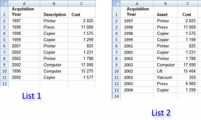
In this example we are going to use two lists with identical columns, shown in the image above. It is easy to modify the COUNTIFS function if your columns are not arranged in the same order, see the COUNTIFS explanation below.
1.1 Create named ranges
There is really no need for named ranges in this example, although they shorten array formulas considerably. You can skip this step if you want.
- Select A2:A13 on sheet "List 2"
- Type Year in Name Box
- Press Enter

Repeat with remaining ranges:
Sheet: List 2 , Range:B2:B13, Name: Asset
Sheet: List 2 , Range:C2:C13, Name: Cost
Sheet: List 1 , Range:A2:A11, Name: Year1
Sheet: List 1 , Range:B2:B11, Name: Asset1
Sheet: List 1 , Range:C2:C11, Name: Cost1
1.2 Filter records existing in only one list

Array formula in cell A4:
To enter an array formula, type the formula in a cell then press and hold CTRL + SHIFT simultaneously, now press Enter once. Release all keys.
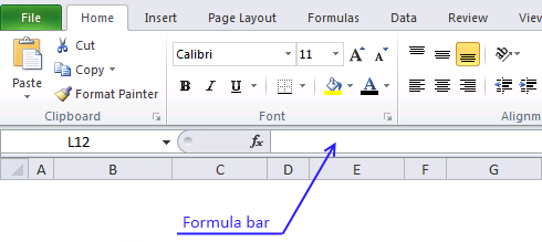
The formula bar now shows the formula with a beginning and ending curly bracket telling you that you entered the formula successfully. Don't enter the curly brackets yourself.
Copy cell A4 and paste it to the right as far as needed. Copy cells and paste down as far as needed.
Array formula in cell A14:
Copy cell A4 and paste it to the right as far as needed. Copy cells and paste down as far as needed.
1.3 Explaining the array formula in cell A4
Step 1 - Find records existing only in List 1
Let us take a look at the bolded part of the formula.
=INDEX('List 1'!$A$2:$C$11, SMALL(IF(COUNTIFS(Year, Year1, Asset, Asset1, Cost, Cost1)=0, ROW(Year1)-MIN(ROW(Year1))+1), ROW(A1)), COLUMN(A1))
COUNTIFS(Year, Year1, Asset, Asset1, Cost, Cost1)
becomes
COUNTIFS({1997, 1998, ... , 1577})
and returns this array: {1, 1, 1, 0, 1, 1, 1, 1, 0, 0}
COUNTIFS(Year, Year1, Asset, Asset1, Cost, Cost1)=0
becomes
{1, 1, 1, 0, 1, 1, 1, 1, 0, 0}=0
and returns
{FALSE, FALSE, FALSE, TRUE, FALSE, FALSE, FALSE, FALSE, TRUE, TRUE}
Step 2 - Convert boolean array to row numbers
The IF function has three arguments, the first one must be a logical expression. If the expression evaluates to TRUE then one thing happens (argument 2) and if FALSE another thing happens (argument 3).
IF(COUNTIFS(Year, Year1, Asset, Asset1, Cost, Cost1)=0, ROW(Year1)-MIN(ROW(Year1))+1)
becomes
IF({FALSE, FALSE, FALSE, TRUE, FALSE, FALSE, FALSE, FALSE, TRUE, TRUE}, {1, 2, 3, 4, 5, 6, 7, 8, 9, 10})
and returns
{FALSE, FALSE, FALSE, 4, FALSE, FALSE, FALSE, FALSE, 9, 10}
Step 3 - Return the k-th smallest value
To be able to return a new value in a cell each I use the SMALL function to filter column numbers from smallest to largest.
The ROW function keeps track of the numbers based on a relative cell reference. It will change as the formula is copied to the cells below.
SMALL(IF(COUNTIFS(Year, Year1, Asset, Asset1, Cost, Cost1)=0, ROW(Year1)-MIN(ROW(Year1))+1), ROW(A1))
becomes
SMALL({FALSE, FALSE, FALSE, 4, FALSE, FALSE, FALSE, FALSE, 9, 10}, 1)
and returns 4.
Step 4 - Return a value of the cell at the intersection of a particular row and column
The INDEX function returns a value based on a cell reference and column/row numbers.
INDEX('List 1'!$A$2:$C$11, SMALL(IF(COUNTIFS(Year, Year1, Asset, Asset1, Cost, Cost1)=0, ROW(Year1)-MIN(ROW(Year1))+1), ROW(A1)), COLUMN(A1))
becomes
=INDEX('List 1'!$A$2:$C$11, 4, COLUMN(A1))
becomes
=INDEX('List 1'!$A$2:$C$11, 4, 1)
and returns 1999.
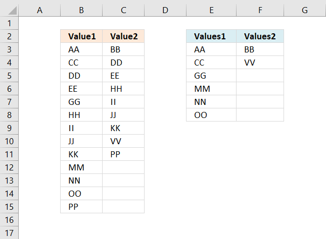
2. Compare two lists and filter unique values where the sum in one column doesn't match the other column
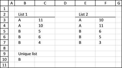
How would you figure out an unique list where the sum of in one column doesn't match the other column? I'm comparing list 1 to list 2
List 1
A 10
A 10
B 5
B 6
B 4
List 2
A 10
A 10
B 5
B 6
Answer is B.
Array formula in cell B10:
2.1 How to enter an array formula
- Select cell B10
- Type the above formula
- Press and hold CTRL + SHIFT simultaneously
- Press Enter once
- Release all keys
If you did it right, the formula is now encapsulated with curly brackets, like this: {formula}
Don´t enter these characters yourself, they show up automatically.
2.2 Explaining the array formula in cell B10
Step 1 - Compare lists
The COUNTIFS function compares column by column between the two lists. If a record is found 1 or more is returned. Nothing found 0 is returned.
COUNTIFS($B$3:$B$7, $E$3:$E$7, $C$3:$C$7, $F$3:$F$7)
returns
{ 1; 1; 1; 1; 0}
Step 2 - Filter only unique distinct values
The COUNTIF function makes sure that only unique distinct values are returned. If a value already exists in the list the function returns 1.
The first argument has a relative and absolute cell reference $B$9:B9. The cell reference expands as you copy and paste the formula further down.
COUNTIF($B$9:B9, $E$3:$E$7)
returns
{0; 0; 0; 0; 0}
This means that no values have been shown yet.
Step 3 - Find the relative position
The MATCH function finds the relative position of the first 0 in the array.
MATCH(0, COUNTIFS($B$3:$B$7, $E$3:$E$7, $C$3:$C$7, $F$3:$F$7) + COUNTIF($B$9:B9, $E$3:$E$7), 0)
becomes
MATCH(0, { 1; 1; 1; 1; 0} + {0; 0; 0; 0; 0}, 0)
becomes
MATCH(0, { 1; 1; 1; 1; 0} , 0)
and returns 5.
Step 3 - Return values
The INDEX function returns a value in a cell range.
INDEX($E$3:$E$7, 5)
becomes
INDEX({"A"; "A"; "B"; "B"; "B"}, 5)
and returns B in cell B10.
Get the Excel file
Compare-two-lists-and-filter-unique-values-where-the-sum-in-one-column-doesn%E2%80%99t-match-the-other-column.xlsx
3. Remove common rows between two Excel defined tables
Sheet 1 and sheet 2 contains random data. As you can see, row 1 and 3 are common records between the two tables.
Sheet1

Sheet2

Count records using COUNTIFS function
- Select cell D2 in sheet1.
- Type
=COUNTIFS(Sheet2!$A$2:$A$4, A2, Sheet2!$B$2:$B$4, B2, Sheet2!$C$2:$C$4, C2)
in cell D2.
- Press Enter

The formula is instantly copied to all table cells in column D. The countifs function counts common records from two tables. Row 2 in sheet1 is found once in sheet 2 and so on.
Hide common rows
- Press with mouse on black arrow

- Deselect 1.
- Press with left mouse button on OK.
Common records are removed.

Repeat steps in Count records using COUNTIFS function and Hide common rows with sheet2.
4. Remove common rows using an array formula between two data sets

This example describes how to compare two tables and extract rows/records not in common using an array formula.
Excel 365 dynamic array formula in cell B15:
The Excel 365 dynamic array formula is entered as a regular formula.
Sheet1

Sheet2

Compare sheet

The following formula is for earlier Excel versions. In contrast to the dynamic array formula above, this formula is required to be entered as an array formula in Excel. The steps are described below. Array formula in cell A2:
This array formula may look complicated but it is not. It contains two different formulas. If the first formula returns an error, the second formula is calculated. The first formula extracts not common rows from the first table. The second formula extracts not common rows from the second table.
You can add a second IFERROR() function to the formula to remove #num errors.
How to create an array formula
- Copy (Ctrl + c) and paste (Ctrl + v) array formula into formula bar.

- Press and hold Ctrl + Shift.
- Press Enter once.
- Release all keys.
Explaining formula
This formula is the first formula. It extracts not common rows from the first table. The second formula is exactly the same but cell references are pointing to the second table.
Step 1 - Identify common records
COUNTIFS(criteria_range1,criteria1, criteria_range2, criteria2...)
Counts the number of cells specified by a given set of conditions or criteria
COUNTIFS(Sheet1!$A$2:$A$4, Sheet2!$A$2:$A$4, Sheet1!$B$2:$B$4, Sheet2!$B$2:$B$4, Sheet1!$C$2:$C$4, Sheet2!$C$2:$C$4)=0
returns {FALSE; TRUE; FALSE}

Step 2 - Convert array into row numbers
IF(COUNTIFS(Sheet1!$A$2:$A$4, Sheet2!$A$2:$A$4, Sheet1!$B$2:$B$4, Sheet2!$B$2:$B$4, Sheet1!$C$2:$C$4, Sheet2!$C$2:$C$4)=0, MATCH(ROW($A$2:$A$4), ROW($A$2:$A$4)), "")
returns {"";2;""}
Step 3 - Return the k-th smallest number
SMALL(array,k) returns the k-th smallest number in this data set.
SMALL(IF(COUNTIFS(Sheet1!$A$2:$A$4, Sheet2!$A$2:$A$4, Sheet1!$B$2:$B$4, Sheet2!$B$2:$B$4, Sheet1!$C$2:$C$4, Sheet2!$C$2:$C$4)=0, MATCH(ROW($A$2:$A$4), ROW($A$2:$A$4)), ""), ROW(A1))
returns 2.
Step 4 - Return a value of the cell at the intersection of a particular row and column
INDEX(array,row_num,[column_num])
Returns a value or reference of the cell at the intersection of a particular row and column, in a given range
INDEX(Sheet1!$A$2:$C$4, SMALL(IF(COUNTIFS(Sheet1!$A$2:$A$4, Sheet2!$A$2:$A$4, Sheet1!$B$2:$B$4, Sheet2!$B$2:$B$4, Sheet1!$C$2:$C$4, Sheet2!$C$2:$C$4)=0, MATCH(ROW($A$2:$A$4), ROW($A$2:$A$4)), ""), ROW(A1)), COLUMN(A1))
returns "Laura" in cell A2.
5. Compare two tables using a condition and filter shared records
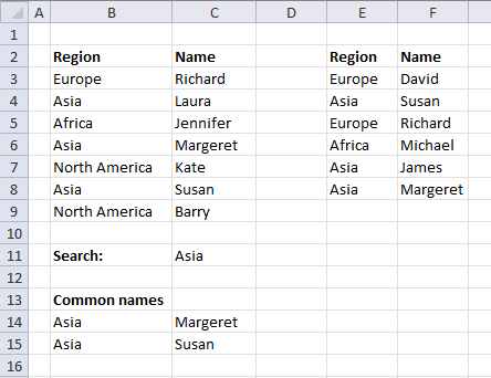
There are two tables on this sheet. The array formula extracts common records in the two tables using a condition. There can be numerous occasions where this can be useful, for example comparing values on the same year or maybe year and month. The picture below shows common names in region Asia.
Excel 365 dynamic array formula i cell B14:
The following formula is created for earlier Excel versions. Array formula in cell B14:
How to enter an array formula
- Select cell B14
- Paste formula to formula bar
- Press and hold CTRL + SHIFT
- Press ENTER
There are now curly brackets surrounding the formula in the formula bar.
Defined tables
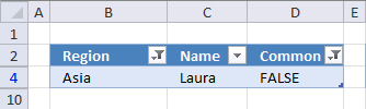
This example demonstrates how to filter not common values in region Asia using defined tables. I converted the two tables to excel defined tables.
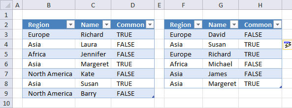
Formula in cell D3:
=COUNTIFS(Table2[[Region ]],B3,Table2[Name],C3)>0
Formula in cell H3:
=COUNTIFS(Table1[Region],F3,Table1[Name],G3)>0
Filter values
- Press with left mouse button on black arrow near header "Common"
- Deselect True
- Press with left mouse button on Ok
- Press with left mouse button on
- Press with left mouse button on black arrow near header "Region"
- Deselect all values except "Asia"
- Press with left mouse button on OK
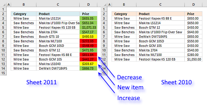
Compare category
This article describes an array formula that compares values from two different columns in two worksheets twice and returns a […]
This article demonstrates techniques to highlight differences and common values across lists. What's on this page How to highlight differences […]
This article demonstrates formulas that extract values that exist only in one column out of two columns. There are text […]
Records category
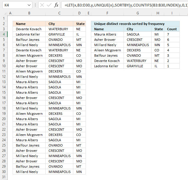
This article demonstrates how to sort records in a data set based on their count meaning the formula counts each […]
Excel categories
12 Responses to “Compare tables: Filter records occurring only in one table”
Leave a Reply
How to comment
How to add a formula to your comment
<code>Insert your formula here.</code>
Convert less than and larger than signs
Use html character entities instead of less than and larger than signs.
< becomes < and > becomes >
How to add VBA code to your comment
[vb 1="vbnet" language=","]
Put your VBA code here.
[/vb]
How to add a picture to your comment:
Upload picture to postimage.org or imgur
Paste image link to your comment.
This is really quality info. Thanks Oscar!!
Julián Fernández,
Thank you for commenting!
Really its super. Thank you !!
Example 1 was more helpful and easy way to identify common and uncommon records... This was really helpful. Thanks a lot !
krishna and Chamundeswari,
Thank you for commenting!
All formulas that belong to you wonderful
Thanks Oscar. Works great. Is there a way to include items that are not in list B in the same formulas. For example C would have avalueof 4 in list A, but it's not in list 2.
Sean,
Thanks Oscar. Works great. Is there a way to include items that are not in list B in the same formulas. For example C would have a value of 4 in list A, but it's not in list 2.
Array formula in cell B10:
=IFERROR(INDEX($E$3:$E$7, MATCH(0, COUNTIFS($B$3:$B$7, $E$3:$E$7, $C$3:$C$7, $F$3:$F$7)+COUNTIF($B$9:B9, $E$3:$E$7), 0)), INDEX($B$3:$B$7, MATCH(0, COUNTIFS($E$3:$E$7, $B$3:$B$7, $F$3:$F$7, $C$3:$C$7)+COUNTIF($B$9:B9, $B$3:$B$7), 0)))
Thanks so much for this invaluable resource, Oscar! I have a question which I don't think is answered by your posts on this topic. Here's an example:
Apples 1
Apples 1
Oranges 2
Apples 3
Apples 3
Bananas 4
Bananas 4
I'm trying to create a formulate that would generate the following list:
Apples
Oranges
Apples
Bananas
That is, I want the formula to use the second column as a criterion for generating the unique list, but the first column as the range for the corresponding values. I hope this is clear, but I'm happy to elaborate if it isn't. Thanks again!
If you want to know more about "Filter a List into unique records using Countif formula", check this link ........
https://www.exceltip.com/excel-filter/filtering-a-list-into-unique-records-using-the-countif-formula.html
HI Oscar, I have almost similar data but in one sheet, seperate with some blank rows, i am trying to extract unique row by comparing both tables but not getting the answer.
Moreover, might possible both table wouldn't have same range, shall thi affect the formula...? TIA
Here is th formula I am trying..
=IFERROR(IFERR0R(INDEX($A$2:$B$7, SMALL(IF(COUNTIFS($A$2:$A$7, $A$11:$A$16, $B$2:$B$7, $B$11:$B$16)=0, MATCH(ROW($A$19:$A$26), ROW($A$19:$A$26)), ""), ROW(A18)), COLUMN(A18)), INDEX($A$11:$B$16, SMALL(IF(COUNTIFS($A$11:$A$16,$A$2:$A$7, $B$11:$B$16,$B$2:$B$7)=0, MATCH(ROW($A$19:$A$26),ROW($A$19:$A$26)), ""), ROW(A18)-SUM(--(COUNTIFS($A$2:$A$7,$A$11:$A$16, $B$2:$B$7,$B$11:$B$16)=0))), COLUMN(A18))), "")
KK,
The following article explains how to extract unique distinct records from two tables:
https://www.get-digital-help.com/extract-unique-distinct-records-from-two-data-sets/