How to highlight differences and common values in lists

This article demonstrates techniques to highlight differences and common values across lists.

1. How to highlight differences in price lists

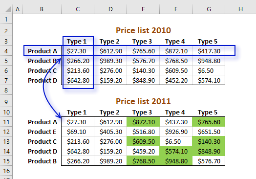
I am now going to show you how to quickly compare two tables using Conditional Formatting (CF). I am going to compare two price lists from the year 2010 and year 2011.

I have two types of data set layouts I want to share a solution for, basic dataset layout shown above and a two-index layout.

To make things more authentic in my examples, products in price list 2011 are not sorted in the same way as 2010. New products are also introduced.

It is quite common that price lists are huge and a total mess. Excel is the perfect tool for finding the differences between datasets.

A requirement for these conditional formatting formulas to work, is that column and row headers have identical spelling.

The same letter capitalization is not required.

1.1Basic dataset layout

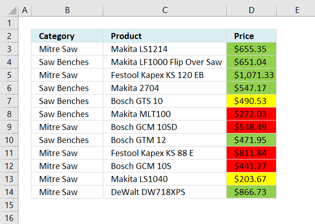
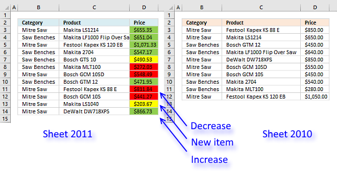
I have two worksheets, in this example, named 2010 and 2011. They both contain a category, product, and a price column.

Color	Description
Yellow	A new item in the list.
Green	Price increase.
Red	Price decrease.

There are three different CF formulas applied to cell range D3:D14, each coloring a cell based on a condition.

Two or more CF formulas can't color cell at the same time, the logical expressions I built can't all be true at the same time.

Red Conditional Formatting formula

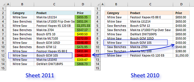
The red CF formula compares the value in column D based on category value and product value with the corresponding product, category and price in worksheet 2010. If the value in column D is smaller the cell is highlighted red.

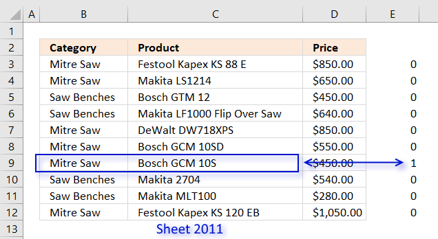
The COUNTIFS function returns an array that indicates the position of the corresponding price. The following explanation is for cell D12, see picture above.

COUNTIFS($B12, 2010'!$B$3:$B$12, $C12, 2010'!$C$3:$C$12) returns {0; 0; 0; 0; 0; 0; 1; 0; 0; 0}.

The MATCH function returns the position of a given value in the array.

MATCH(1,COUNTIFS($B12, 2010'!$B$3:$B$12, $C12, 2010'!$C$3:$C$12), 0)

becomes

MATCH(1,{0; 0; 0; 0; 0; 0; 1; 0; 0; 0}, 0) and returns 7. Now we know where the value we are looking for is.

$D12<INDEX(2010'!$D$3:$D$12, MATCH(1,COUNTIFS($B12, 2010'!$B$3:$B$12, $C12, 2010'!$C$3:$C$12), 0))

becomes

$D12<INDEX(2010'!$D$3:$D$12, 7)

becomes

$441.27<$450 and returns TRUE.

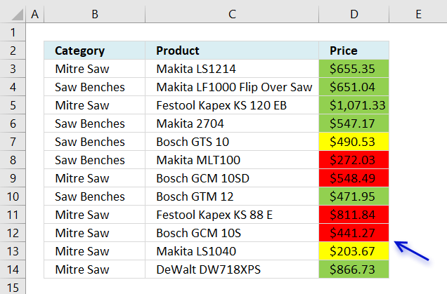
Cell D12 is highlighted red.

Back to top

Green Conditional Formatting formula

The green CF formula is similar to the red CF formula except that the cell is highlighted green if the value in column D is larger than the corresponding value in worksheet 2010.

The only difference between the red and green CF formulas is the larger than and smaller than sign.

Back to top

Yellow Conditional Formatting formula

The yellow CF formula checks if the category and product is not found in worksheet 2010, if TRUE the cell is highlighted yellow.

Back to top

Back to top

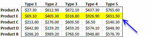
Two index table

The questions I am going to answer in this article are:

• How do I find new products or models compared to previous year?
  
• How to identify lowered prices compared to previous year?
  
• How to identify higher prices compared to previous year?
  

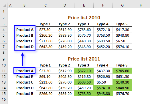
Here are the two tables together on the same worksheet.

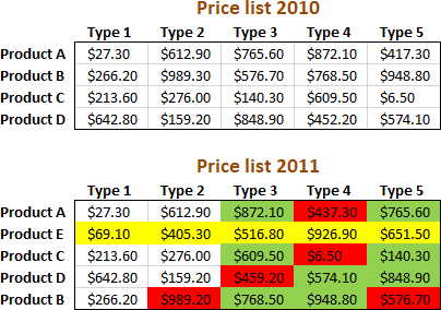
As you can see "product E" is new for 2011 (highlighted yellow), "product A" type 4 has a lower price than the previous year 2010 (highlighted red), etc.

The colors make it very easy to spot differences.

Back to top

New values compared to last year

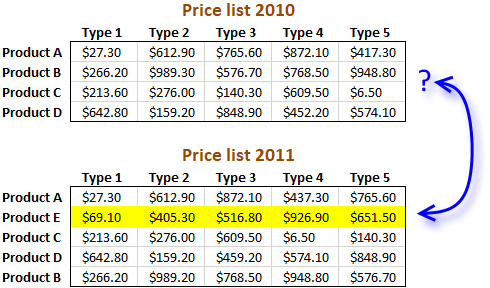
The following CF formula highlights entire row yellow if it finds a new product name.

Conditional formatting formula:

It compares the product and type columns between the tables and if a value is not found the CF formula highlights the entire row yellow.

Back to top

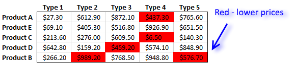
Find lower prices

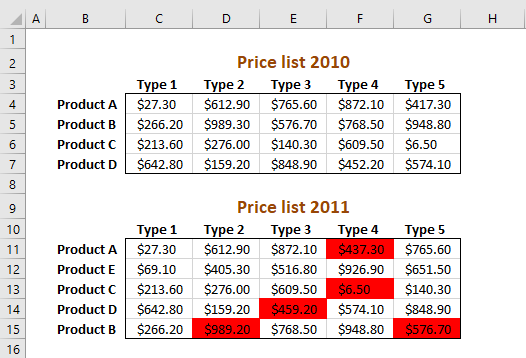
Conditional formatting formula:

Cells are formatted red if the price is lower than the price in the other table.

Back to top

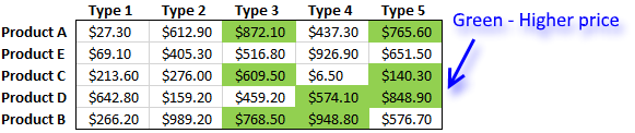
Find higher prices

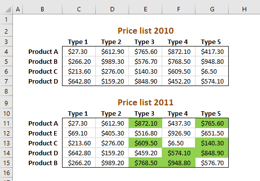
Conditional formatting formula:

Cells are formatted green if the price is higher than the price in the other table.

Back to top

How to apply conditional formatting formula

Make sure you adjust cell references to your excel sheet.

1. Select cells C11:G15
2. Press with left mouse button on "Home" tab
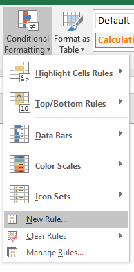
3. Press with left mouse button on "Conditional Formatting" button
4. Press with left mouse button on "New Rule.."
5. Press with left mouse button on "Use a formula to determine which cells to format"
6. Copy and paste conditional formatting formula in "Format values where this formula is TRUE" window.
7. Press with left mouse button on "Format.." button
8. Press with left mouse button on "Fill" tab
9. Select a color for highlighted cells.
10. Press with left mouse button on "Ok"
11. Press with left mouse button on "Ok"
12. Press with left mouse button on "Ok"

Back to top

Explaining find lower prices conditional formatting formula in cell C11

You can follow along, copy the CF formula and paste it in a cell.

Go to tab "Formula" on the ribbon and then press with left mouse button on "Evaluate Formula" button.

Press with mouse on the "Evaluate" button to move to the next step in the calculations.

Step 1 - Find relative position of current row header in previous pricelist

=INDEX($C$4:$G$7, MATCH($B11, $B$4:$B$7, 0), MATCH(C$10, $C$3:$G$3, 0))<C11

The MATCH function returns the relative position of an item in an array that matches a specified value.

MATCH($B11, $B$4:$B$7, 0)

becomes

MATCH("Product A", {"Product A";"Product B";"Product C";"Product D"}, 0)

and returns 1.

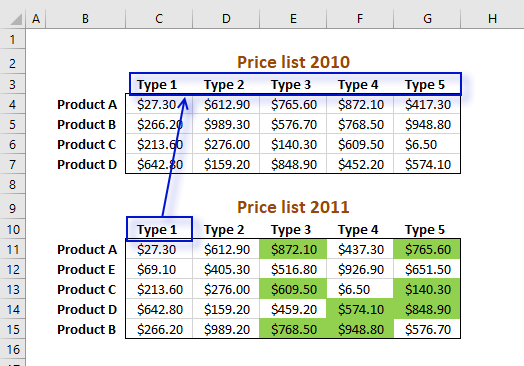
Step 2 - Find relative position of current column header in previous price list

=INDEX($C$4:$G$7, MATCH($B11, $B$4:$B$7, 0), MATCH(C$10, $C$3:$G$3, 0))<C11

MATCH(C$10, $C$3:$G$3, 0)

becomes

MATCH("Model 1", {"Model 1", "Model 2", ... , "Model 5"}, 0)

returns 1. Type 1 is found in position 1 in cell range C3:G3.

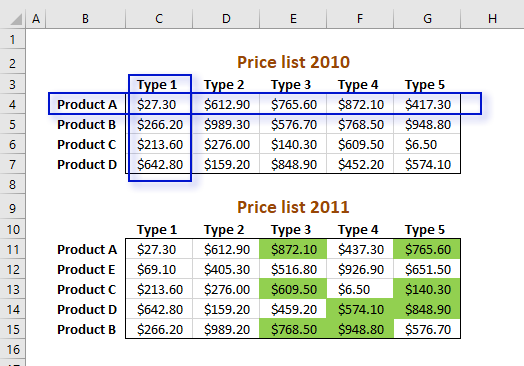
Step 3 - Return a value of the cell at the intersection of a particular row and column

=INDEX($C$4:$G$7, MATCH($B11, $B$4:$B$7, 0), MATCH(C$10, $C$3:$G$3, 0))<C11

returns 27,3. The picture above shows how the formula finds the value at the intersection of a given row and column number.

Step 4 - Compare returned value to current value

=INDEX($C$4:$G$7, MATCH($B11, $B$4:$B$7, 0), MATCH(C$10, $C$3:$G$3, 0))<C11

becomes

27,3>C11

becomes

27,3>27,3

returns FALSE. Cell C11 is not highlighted green.

Back to top

Get Excel *.xlsx file

compare price lists.xlsx

Back to top

2. Compare two columns and highlight differences

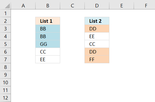
This section demonstrates a conditional formatting formula that will highlight the differences between two columns. The image above shows two cell ranges containing values, the first one is in column B and the second one is in column D.

Values "BB", "GG", and "GG" are highlighted, they only exist in column B. Values "DD" and "FF" are highlighted, they only exist in column D.

Conditional formatting is a built-in feature that allows you to format specific cells based on a condition or criteria.

The conditional formatting formula presented in this article highlights values that only exist in one column, in other words, they differ from the values in the other column. You can pick any format or fill color and the formula lets you build advanced criteria that must be met.

2.1 How to highlight values

1. Select cell range B3:B7.
2. Go to tab "Home" on the ribbon if you are not there already.
3. Press with mouse on the Conditional Formatting button.
4. Press with mouse on "New Rule...".
   
5. Press with mouse on "Use a formula to determine which cells to format".
6. Type: =AND($D$3:$D$7<>B3)
7. Press with mouse on "Format..." button.
8. Press with mouse on "Fill" tab.
9. Pick a color.
10. Press with left mouse button on OK.
11. Press with left mouse button on OK.

Repeat above steps with column D, the formula is =AND($B$3:$B$7<>D3)

2.2 Explaining conditional formatting formula

Step 1 - Check if cell range D3:D7 is not equal to cell B3

Reference $D$3:$D$7 is an absolute cell reference meaning it is locked, it won't change when the CF moves to the next cell.

The less than and larger than sign combined means not equal to.

$D$3:$D$7<>B3

becomes

$D$3:$D$7<>B3

and returns {TRUE; TRUE; TRUE; TRUE; TRUE}.

Step 2 - Check if all boolean values are TRUE

AND($D$3:$D$7<>B3)

AND($D$3:$D$7<>B3)

becomes

AND({TRUE; TRUE; TRUE; TRUE; TRUE})

and returns TRUE. Cell B3 is highlighted.

2.3 Get Excel *.xlsx

Compare two columns and highlight differences.xlsx

3. Compare two columns and highlight values in common

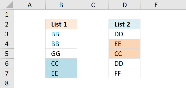
A conditional formatting formula highlights values in column B that also exist in column D.

The same thing happens in column D, a conditional formatting formula highlights values in common between column B and D.

How to highlight common values

1. Select cell range B3:B7
2. Go to tab "Home" on the ribbon if you are not there already
3. Press with mouse on Conditional Formatting button
4. Press with mouse on "New Rule..."
   
5. Press with mouse on "Use a formula to determine which cells to format"
6. Type: = COUNTIF($D$3:$D$7, B3)
   
7. Press with mouse on "Format..." button
8. Press with mouse on "Fill" tab.
9. Pick a color
10. Press with left mouse button on OK
11. Press with left mouse button on OK

Repeat above steps with column D, the formula is at the top of this article.

Explaining conditional formatting formula

The COUNTIF function counts how many times value in cell B3 is found in cell range $D$3:$D$7. B3 changes to B4 when Excel moves on to next cell below, however, that is not the case with $D$3:$D$7.

The $ dollar signs make this cell reference locked, in other words, it doesn't change.

The Conditional Formatting in Excel interprets all numbers except 0 as TRUE so if the COUNTIF function finds a value twice and returns 2 doesn't matter, it still highlights the cell.

Get excel *.xlsx file

Compare two columns and highlight matches.xlsx

This blog article is one out of five articles on the same subject.

• Filter values existing in range 1 but not in range 2 using array formula in excel
• Filter common values between two ranges using array formula in excel
• How to remove common values between two columns
• How to find common values from two lists
• Highlight common values in two lists using conditional formatting in excel

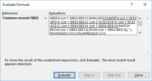
4. Compare two lists of data and highlight common records

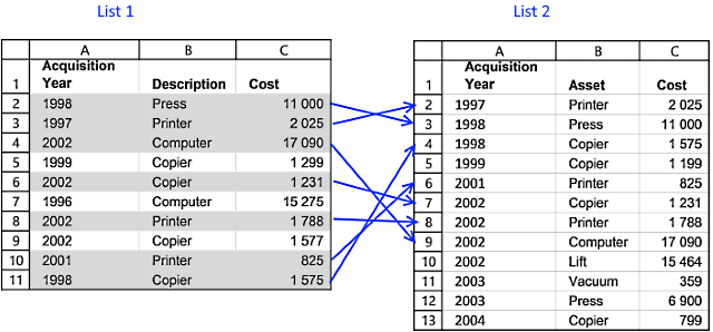
In this blog post I will demonstrate a conditional formatting formula that will highlight common records in two lists. The image above shows you highlighted records in List 1 that also exists in sheet2.

You can also use a formula to extract shared records or an Excel defined table, if you prefer that. There is also an article written for Comparing two columns and highlight values in common.

There are more links to related articles in the sidebar.

Create named ranges

When constructing a conditional formatting formula you can only reference cells on current sheet. But there is a workaround. The answer is named ranges.

Here is how to create named ranges for this example:

1. Go to sheet List 2
2. Select cell range A2:A13
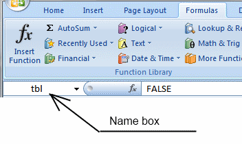
3. Press with left mouse button on in Name box
4. Type a name (Year)
5. Repeat step 1 to 4 with remaining columns.

Setup COUNTIFS function

The COUNTIFS function looks for duplicate records in the second list (List 2).

COUNTIFS(criteria_range1,criteria1, criteria_range2, criteria2...)
Counts the number of cells specified by a given set of conditions or criteria

In this example:
List 1:Column A - List 2: Column A (Year)
List 1:Column B - List 2: Column B (Asset)
List 1:Column C - List 2: Column C (Cost)

COUNTIFS(YEAR, $A2, ASSET, $B2, COST, $C2)

This formula contains absolute and relative cell references. The conditional formatting formula must look for values in matching columns.

$A2 is a cell reference to values in column A. The column ($A) is absolute but the row (2) is relative. When the conditional formatting formula runs the next row, only the row number changes, example $A3. The named ranges do not change.

If the COUNTIFS function finds one matching record it returns 1, if nothing is found 0 (zero) is returned. 0 (zero) is the equivalent to FALSE so the Conditional formatting will not highlight a cell i FALSE is returned.

Highlight common records from two lists Excel 2007

How to apply conditional formatting formula:

1. Select cells A2:C11 (Sheet: List 1)
2. Press with left mouse button on "Home" tab
3. Press with left mouse button on "Conditional Formatting" button
4. Press with left mouse button on "New Rule.."
5. Press with left mouse button on "Use a formula to determine which cells to format"
6. Type =COUNTIFS(YEAR, $A2, ASSET, $B2, COST, $C2) in "Format values where this formula is TRUE" window.
   
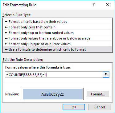
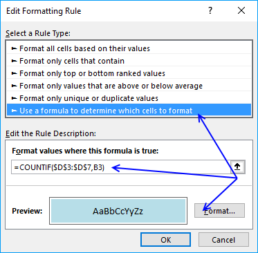
   (The formula shown in the image above is not used in this article)
7. Press with left mouse button on "Format.." button
8. Press with left mouse button on "Fill" tab
9. Select a color for highlighting cells.
10. Press with left mouse button on "Ok"
11. Press with left mouse button on "Ok"
12. Press with left mouse button on "Ok"

Highlight common records from two lists Excel 2003

Conditional formatting formula:

5. Compare two tables and highlight differences

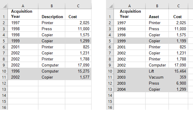
The image above demonstrates a conditional formatting formula that highlights records that only exist in one table. There are two tables in this example: List 1 and List 2.

If you are looking for a conditional formatting formula that highlights records shared by both tables: Compare tables: Highlight common records. There is also an article that demonstrates how to filter records not in both tables.

The conditional formatting formula does not work with cell references outside the current sheet so we need to rely on named ranges for this to work.

Create named ranges

1. Select A2:A13 on sheet "List 2"
2. Type Year in Name Box
3. Press Enter

Repeat with remaining ranges:
Sheet: List 2 , Range:B2:B13, Name: Asset
Sheet: List 2 , Range:C2:C13, Name: Cost
Sheet: List 1 , Range:A2:A11, Name: Year1
Sheet: List 1 , Range:B2:B11, Name: Asset1
Sheet: List 1 , Range:C2:C11, Name: Cost1

Highlight records existing in only one list

How to apply conditional formatting formula:

Sheet: List 1

1. Select cells A2:C11 (Sheet: List 1)
2. Press with left mouse button on "Home" tab
3. Press with left mouse button on "Conditional Formatting" button
4. Press with left mouse button on "New Rule.."
5. Press with left mouse button on "Use a formula to determine which cells to format"
6. Type =COUNTIFS(Year, $A2, Asset, $B2, Cost, $C2)=0 in "Format values where this formula is TRUE" window.
   
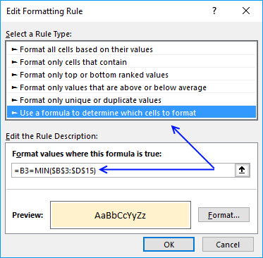
   (The formula displayed in the image above is not used in this article)
7. Press with left mouse button on "Format.." button
8. Press with left mouse button on "Fill" tab
9. Select a color for highlighting cells.
10. Press with left mouse button on "Ok"
11. Press with left mouse button on "Ok"
12. Press with left mouse button on "Ok"

Sheet: List 2

1. Select cells A2:C13 (Sheet: List 2)
2. Press with left mouse button on "Home" tab
3. Press with left mouse button on "Conditional Formatting" button
4. Press with left mouse button on "New Rule.."
5. Press with left mouse button on "Use a formula to determine which cells to format"
6. Type =COUNTIFS(Year1, $A2, Asset1, $B2, Cost1, $C2)=0 in "Format values where this formula is TRUE" window.
   
   (The formula displayed in the image above is not used in this article)
7. Press with left mouse button on "Format.." button
8. Press with left mouse button on "Fill" tab
9. Select a color for highlighting cells.
10. Press with left mouse button on "Ok"
11. Press with left mouse button on "Ok"
12. Press with left mouse button on "Ok"

Highlight records existing in only one list, excel 2003

The COUNTIFS function was introduced in Excel 2007 and if you have an earlier version you need another formula shown below. The COUNTIF functions returns arrays that are multiplied, the SUMPRODUCT function then adds the numbers and returns a total.

Sheet: List 1

Conditional formatting formula:

Sheet: List 2

Conditional formatting formula:

Sheet: List 1

Sheet: List 2

Recommended reading

Built-in conditional formatting

Data Bars Color scales Icons

Highlight cells rule

Highlight cells containing string
Highlight a date occuring
Conditional Formatting Basics
Highlight unique/duplicates

Top bottom rules

Highlight top 10 values
Highlight top 10 % values
Highlight above average values

Basic CF formulas

Working with Conditional Formatting formulas
Find numbers in close proximity to a given number
Highlight empty cells
Highlight text values

Search using CF

Highlight records – multiple criteria [OR logic]
Highlight records [AND logic]
Highlight records containing text strings (AND Logic)
Highlight lookup values

Unique distinct

How to highlight unique distinct values
Highlight unique values and unique distinct values in a cell range
Highlight unique values in a filtered Excel table
Highlight unique distinct records

Duplicates

How to highlight duplicate values
Highlight duplicates in two columns
Highlight duplicate values in a cell range
Highlight smallest duplicate number
Highlight more than once taken course in any given day
Highlight duplicates with same date, week or month
Highlight duplicate records
Highlight duplicate columns
Highlight duplicates in a filtered Excel Table

Compare

Highlight missing values between to columns
Compare two columns and highlight values in common
Compare two lists of data: Highlight common records
Compare tables: Highlight records not in both tables
How to highlight differences and common values in lists
Compare two columns and highlight differences

Min max

Highlight smallest duplicate number
How to highlight MAX and MIN value based on month
Highlight closest number

Dates

Advanced Date Highlighting Techniques in Excel
How to highlight MAX and MIN value based on month
Highlight odd/even months
Highlight overlapping date ranges using conditional formatting
Highlight records based on overlapping date ranges and a condition
Highlight date ranges overlapping selected record [VBA]
How to highlight weekends [Conditional Formatting]
How to highlight dates based on day of week
Highlight current date

Misc

Highlight every other row
Dynamic formatting
Advanced Techniques for Conditional Formatting
Highlight cells based on ranges
Highlight opposite numbers
Highlight cells based on coordinates

Excel categories

Comments (6)