How to use the CUMIPMT function
What is the CUMIPMT function?
The CUMIPMT function calculates the accumulated interest based on a start and end period on a loan.
Table of Contents
1. Introduction
What is accumulated interest?
Accumulated interest refers to the total amount of interest earned on an investment or paid on a loan up to a specified date. This process of interest earning interest is called compounding.
What is a loan?
A loan is an amount of money you borrow from an individual or entity. The lender is usually a corporation, financial institution, or government, however it can also be an individual. A lender is an entity or individual that makes funds available for a borrower that can be a person or a business. The borrower agrees to repay the loan amount plus interest over an agreed-upon period of time.
What are the start and end period on a loan?
The start period or start date is the date the loan begins and interest accrual starts. The end period or maturity date is the final due date when the loan must be fully repaid.
The CUMIPMT function lets you calculate the accumulated interest based on a start and end date, however, these dates must not necessarily be the start and end date of the loan.
For example, a loan is to be repaid after 5 years. The CUMIPMT function lets you calculate the accumulated interest between year 3 and 4.
What is an annuity loan?
An annuity loan is a type of loan where the borrower makes equal periodic payments (usually monthly or annually) over a fixed term. These periodic payments consist of both principal and interest components. The interest is calculated based on the outstanding loan balance, and the principal repayment portion gradually increases over time as the interest portion decreases.
2. CUMIPMT function Syntax
CUMIPMT(rate, nper, pv, start_period, end_period, type)
| rate | Required. The interest rate. |
| nper | Required. The total number of periods in an annuity.
Examples: |
| pv | Required. Present value. |
| start_period | Required. The first period. |
| end_period | Required. The last period. |
| type | Required. When payments are due.
0 - End of period. |
What is an annuity?
An annuity is a series of equal payments made over a defined period of time. The payments are usually made monthly, quarterly, or annually. These payment intervals are the "periods" that nper counts.
For example, if an annuity pays out quarterly for 3 years, there would be:
4 payments per year
3 years
So nper = 4 * 3 = 12 total payment periods
What is interest rate?
A fixed interest rate is an interest rate that remains the same throughout the term of a loan or an investment.
What is a monthly payment?
A monthly payment is a scheduled payment that occurs every month as part of an ongoing loan, mortgage, or other finance agreement.
What is a quarterly payment?
A quarterly payment is a scheduled payment that occurs every quarter as part of an ongoing loan, mortgage, or other finance agreement.
3. Example 1

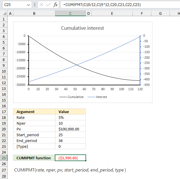
You take out a $100,000 mortgage loan at 5% annual interest rate for 10 years with monthly payments. Calculate the cumulative interest paid during year 3?
The arguments are:
| Rate | 5% |
| Nper | 10 |
| Pv | $100,000.00 |
| Start_period | 25 |
| End_period | 36 |
| [Type] | 0 |
The image above shows the CUMIPMT function in cell E25 calculating the accumulated interest for month 25 to 36 for a 10 year loan of $100 000 based on a 5% interest. Year 3 corresponds to months 25 to 36, the type is 0 (zero) meaning the payments are due at the end of the period.
The first argument is the interest rate per year, we calculate the interest on a monthly basis so the argument has to be divide with 12, there are 12 months in a year.
The second argument is the number of periods the interest is calculated for, 10 year * 12 = 120 months or periods.
Formula in cell E3:
The formula returns -$3,990.60 which represents the accumulated interest between months 25 to 36. The chart above has a primary and secondary axis, it shows the interest paid for each period (orange curve). It decreases until the loan is repaid and corresponds to the right y-axis. The gray curve represents the cumulative interest paid and it corresponds to the left y-axis.
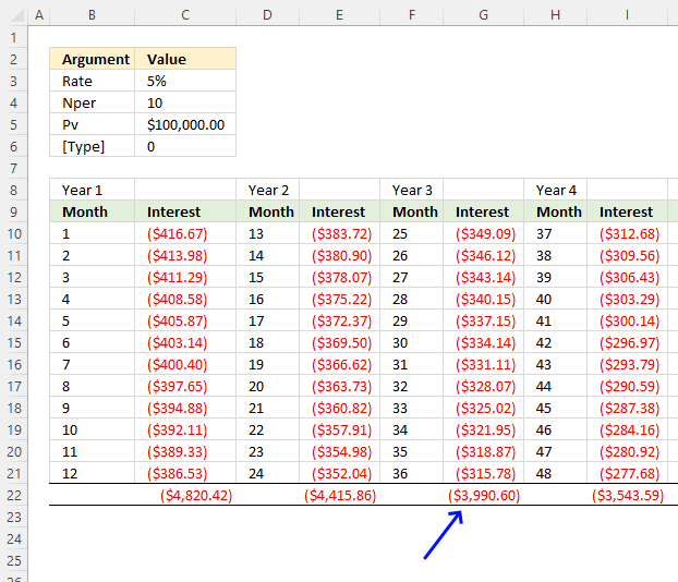
This image shows the interest for months 25 to 36 and the cumulative interest. The amount in cell G22 is the same as in the top image cell E3.
4. Example 2
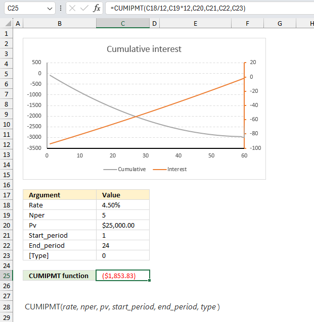
A car loan of $25,000 is taken at 4.5% annual interest rate for 5 years with monthly payments. Find the total interest paid in the first 2 years of the loan?
The arguments are:
| Rate | 4.5% |
| Nper | 5 |
| Pv | $25,000.00 |
| Start_period | 1 |
| End_period | 24 |
| [Type] | 0 |
The image above shows the CUMIPMT function in cell E25 calculating the accumulated interest for month 1 to 24 for a 5 year car loan of $25,000 based on a 4.5% interest. The first two years correspond to months 1 to 24, the type is 0 (zero) meaning the payments are due at the end of the period.
Formula in cell C25:
The formula returns -$1853.83 which represents the accumulated interest for months 1 to 24. The chart above has a primary and secondary axis, it shows the interest paid for each period (orange curve). It decreases until the loan is repaid and corresponds to the right y-axis. The gray curve represents the cumulative interest paid and it corresponds to the left y-axis.
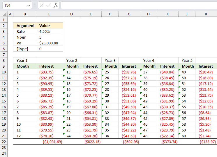
The image above shows a table containing the interest paid for each month divided into years. 1,031.69 is paid in year 1, 822.15 is paid in year 2. The total is 1,031.69 + 822.15 equals 1853.83 which is the same values in cell C25 shown in the image before.
5. Example 3
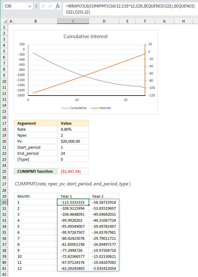
You take out a $20,000 loan at 6.8% annual interest rate for 2 years with monthly payments. Create a data set containing the interest paid for each month.
The arguments are:
| Rate | 6.80% |
| Nper | 2 |
| Pv | $20,000.00 |
| Start_period | 1 |
| End_period | 24 |
| [Type] | 0 |
Excel 365 dynamic array formula in cell C25:
This formula creates an array of values containing all interests paid between month 1 and 24. This means that if you change the arguments in C18:C23 the data table changes accordingly. It grows if you specify a Nper value larger than 2 and shrinks if smaller than 2.
The calculation in cell C25 calculates all values in one formula, the output spills too cells below and to the right as far as needed.
Explaining formula
Step 1 - Create a sequence
The SEQUENCE function creates a list of sequential numbers.
Function syntax: SEQUENCE(rows, [columns], [start], [step])
SEQUENCE(C19*12)
becomes
SEQUENCE(24)
and returns
{1; 2; 3; ... ; 24}
Step 2 - Calculate interest for each month
The CUMIPMT calculates interest values based on the sequence from 1 to 24 we created above. The sequence numbers represent month numbers.
CUMIPMT(C18/12,C19*12,C20,SEQUENCE(C19*12),SEQUENCE(C19*12),C23)
returns
{-113.333333333333;-108.911599443412; ... ;-5.03542205383826}
Step 3 - Wrap array to 12 rows representing months
The WRAPCOLS function rearranges values from a single row to a 2D cell range based on a given number of values per column.
Function syntax:
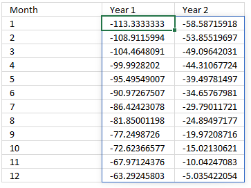
WRAPCOLS(CUMIPMT(C18/12,C19*12,C20,SEQUENCE(C19*12),SEQUENCE(C19*12),C23),12)
returns the array divided into 12 months:
6. CUMIPMT function not working
The CUMIPMT function returns
- #NUM error value if:
- rate <= 0
- nper <= 0
- pv <= 0
- start_period < 1
- end_period < 1
- start_period > end_period
- type is not 0 (zero) or 1
Use the same unit for rate and nper, the above example uses monthly payments. That is why the interest rate is divided by 12 and nper is multiplied by 12. There are 120 monthly payments in a 10-year period.
Functions in 'Financial' category
The CUMIPMT function function is one of 27 functions in the 'Financial' category.
How to comment
How to add a formula to your comment
<code>Insert your formula here.</code>
Convert less than and larger than signs
Use html character entities instead of less than and larger than signs.
< becomes < and > becomes >
How to add VBA code to your comment
[vb 1="vbnet" language=","]
Put your VBA code here.
[/vb]
How to add a picture to your comment:
Upload picture to postimage.org or imgur
Paste image link to your comment.
Contact Oscar
You can contact me through this contact form