How to use the PMT function
What is the PMT function?
The PMT function returns the payment amount needed for borrowing a fixed sum of money based on constant payments (annuity) and interest rate.
You can also use the PMT function to calculate the amount to save each period to reach a given sum, based on an interest rate and the number of periods.
Table of Contents
1. Introduction
What is the principal?
The principal is the amount you have to pay back and interest is the charges you pay for borrowing the money.
What is an investment?
An investment is an asset or business acquired with the goal of generating income or appreciation, the purpose is to grow the money over time.
What are periods?
A payment period is the length of time between payments made on a loan or investment. For example, a loan with monthly payments the payment period would be one month. A loan with quarterly payments the payment period would be three months.
What is present value?
The present value is the initial amount that will earn interest/dividend.
What is future value?
The compounded amount after the calculated periods based on the given rate. It measures what a current capital (present value) amount will be worth at a designated future date.
What are periodic constant payments?
Periodic constant payments are payments that are made at regular intervals such as monthly, quarterly, or yearly and have the same amount each time.
What is a constant interest rate?
A fixed interest rate is an interest rate that remains the same throughout the term of a loan or an investment.
What is the number of compounding periods per year?
The number of compounding periods per year refers to how often interest is compounded annually on an investment or loan.
Some common compounding periods:
- Annually - 1 compounding period per year
- Semiannually - 2 compounding periods per year
- Quarterly - 4 compounding periods per year
- Monthly - 12 compounding periods per year
- Weekly - 52 compounding periods per year
- Daily - 365 compounding periods per year
What is compounding?
Compounding refers to the process of generating more interest from interest that was previously earned. It causes interest to grow exponentially over time.
Related functions
| Function | Description |
|---|---|
| PMT(rate, nper, pv, [fv], [type]) | Returns the payment amount needed for borrowing a fixed sum of money based on constant payments (annuity) and interest rate. |
| PPMT(rate, per, nper, pv, [fv], [type]) | Calculates the principal payment for a specific period for an investment based on repeated constant payments and a constant interest rate. |
| IPMT(rate, per, nper, pv, [fv], [type]) | Calculates the interest payment for a specific period for an investment based on repeated constant payments and a constant interest rate. |
| ISPMT(rate, per, nper, pv) | Calculates the interest paid during a specific period of an investment. |
2. Syntax
PMT(rate, nper, pv, [fv], [type])
| Rate | Required. The interest rate. |
| nper | Required. The number of payments. |
| pv | Required. The present value. |
| [fv] | Optional. The future value. Default value is 0 (zero). |
| [type] | Optional. When payments are due, default value is 0 (zero).
0 (zero) : at the end of the period. 1 : at the beginning of the period. |
Think carefully about what period you use (years, quarterly, months, weekly, days or whatever unit) before you specify the number of payments (nper) and the interest rate.
Monthly payments: For a ten-year loan at an annual interest rate of 5 percent use 5%/12 (rate) and 10*12 (nper).
Annual payments: For a ten-year loan at an annual interest rate of 5 percent use 5% (rate) and 10 (nper).
3. Example 1

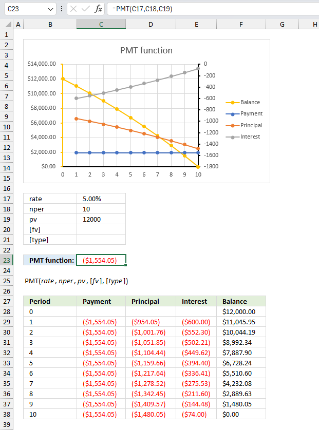
What annual payment is needed for a $12,000 10-year loan that covers both interest and principal?
The above image shows the annual payment needed for a 10-year $12,000 loan based on a 5 percent interest rate.
The provided arguments are:
- Rate: This is the interest rate per period. In the example, it is set to 5%.
- Nper: This is the total number of periods for the loan or investment. In the example, it is set to 10 periods (years).
- Pv: This is the present value or the initial loan amount. In the example, it is set to $12,000.00.
- [fv] (optional): This is the future value or the remaining balance after the last payment. In the example, it is left blank, assuming a future value of 0 (the loan is fully paid off).
- [Type] (optional): 0 This is the timing of the payments (0 for payments due at the end of the period, 1 for payments due at the beginning of the period). If left blank, assuming the default end-of-period payment.
Formula in cell C23:
The formula in cell C23 returns $1,554.05 which represents the payment needed to cover both the principal and the interest for a annuity loan over 10 years with an interest rate of 5%.
The chart displays the periodic loan payment for a given principal amount, interest rate, and number of periods (nper). The x-axis represents the period numbers from 0 to 10, while the y-axis shows the dollar amounts.
- The yellow curve represents the outstanding balance, which starts at $12,000 (the initial principal amount) and decreases over time as payments are made.
- The orange curve represents the periodic payment amount, which remains constant at $1,554.05 throughout the loan term.
- The blue curve shows the principal portion of each payment, which gradually increases over time.
- The gray curve represents the interest portion of each payment, which decreases over time as the outstanding balance decreases.
The data table at the bottom provides the numerical values for each period, including the payment amount, principal portion, interest portion, and remaining balance after each payment. The chart demonstrates how the PMT function calculates the fixed periodic payment and how that payment is split between principal and interest components over the loan term with the balance gradually decreasing until it reaches zero at the end.
4. Example 2
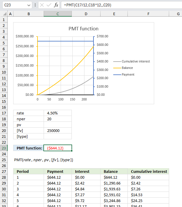
You want to save $250,000 for retirement by making monthly deposits into an account earning 4.5% annual interest. You have 20 years to retirement, how much do you need to save each month to reach your goal?
This example demonstrates how to calculate the monthly savings amount needed to reach 2,500,000 with a 4.5% interest rate and 20 years of savings.
The provided arguments are:
- Rate: This is the interest rate per period. In the example, it is set to 4.5%. We are going to use months as periods so we need to calculate the ratio between 4.5% and 12.
- Nper: This is the total number of periods for the loan or investment. In the example, it is set to 20 periods (years). However, the fomrula multiples this value with 12 because there are 12 months in a year.
- Pv: In the example, it is left blank, assuming the present value of 0 (zero).
- [fv] (optional): This is the future value or the remaining balance after the last payment. In the example, it is set to $2,500,000.00.
- [Type] (optional): 0 This is the timing of the payments (0 for payments due at the end of the period, 1 for payments due at the beginning of the period). If left blank, assuming the default end-of-period payment.
Formula in cell C23:
The formula in cell C23 returns $644.12 which represents the payment needed to reach a future value of 2,500,00 based on 20 years of savings and an annual interest rate of 4.5%.
The chart above shows the balance, payment each month, and the cumulative interest earned over 20 years.
5. Excel Annuity Loan Calculator
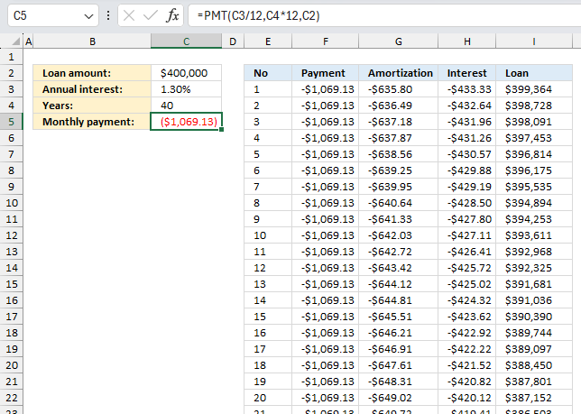
The image above describes an annuity loan calculator that you can find in the attached file at the end of this article. The picture displays payment, amortization or principal, interest, and remaining loan per month based on your input values in cells:
- C2 - this is the loan amount.
- C3 - annual interest rate
- C4 - number of years to repay the loan amount
- C5 - this is not an input value. Excel calculates this value for you. Section 5.1 below describes this formula in great detail.
| Loan amount | This is the total amount you borrow, this can be, for example, a mortgage. |
| Annual interest | A percentage that you will pay for the loan annually. |
| Years | For how long the loan will be paid. |
| Monthly payment | This cell is calculated by Excel using the PMT function, don't enter a value here. |
The formulas in columns E, F, G, H and I resize appropriately based on the values you enter in C2:C4. The calculator returns:
- the number of months (periods) in column E
- the equal payments amount in column F
- the amortization or principal in column G
- the interest in column H
- the loan balance in column I
5.1 Calculate the monthly payment

The first thing this loan calculator does is to determine the monthly payment for the given inputs in cells C2, C3, and C4. This amount is then used in column F.
Formula in cell C5:
An annuity loan lets you pay equal amounts in regular intervals, the formula in cell C5 calculates this amount for you. The following steps describe in great detail how the formula works.
Explaining formula in cell E4
Step 1 - Calculate yearly payment
The PMT function has the following arguments: PMT(rate, nper, pv, [fv], [type])
rate - interest rate. We need to divide the annual interest rate with the number of monts in a year. C3/12
nper - number of payments. We are paying this on a monthly basis, 40 year * 12 months = 480 periods.
pv - present value. This value is 400,000.
PMT(C3/12,C4*12,C2) returns -1069.13
5.2 Create a sequence of numbers representing months

The following formula creates an array of numbers from 1 to the calculated number of periods. This example has 40 years and there are 12 months in a year. 40 * 12 = 480.
Excel 365 dynamic array formula in cell E3:
The formula above returns an array containing number from 1 to n where n is the number of periods. This formula works only in Excel 365 and it spills values to cell E3 and cells below as far as needed. This makes the loan calculator dynamic meaning it adjusts to the input values in cells C2, C3, and C4 automatically.
Explaining formula in cell E4
Step 1 - Calculate months needed to pay back loan
C4*12
becomes
40*12 equals 480.
Step 2 - Create sequence
The SEQUENCE function creates a list of sequential numbers.
Function syntax: SEQUENCE(rows, [columns], [start], [step])
SEQUENCE(C4*12)
becomes
SEQUENCE(480)
and returns {1;2;3; ... ; 480}
5.3 Populate column F with payments

The following formula populates the appropriate number of cells from F2 to cells below as far as needed with the monthly payment amount.
Formula in cell F3:
The formula above returns an array as large as the sequence for periods, it contains the payment amount. This formula works only in Excel 365 and it spills values to cell F3 and cells below as far as needed. This makes the loan calculator dynamic meaning it adjusts to the input values in cells C2, C3, and C4 automatically.
Explaining formula in cell F3
Step 1 - Calculate monthly payment
The cell references below are absolute cell references, they don't change when we copy the cell and paste to cells below.
PMT(C3,C4,C2)/12
becomes
PMT(0.013, 40, 400000)/12
and returns -1069.13
Step 2 - Divide with 12
The asterisk lets you multiply values in an Excel formula.
C4*12 becomes 40*12 and returns 480
Step 3 - Increase array size
The EXPAND function increases a cell range or array by a specified number of columns and rows.
Function syntax:
EXPAND(PMT(C3,C4,C2)/12,C4*12,,PMT(C3,C4,C2)/12)
becomes
EXPAND(-1069.13,C4*12,,-1069.13)
and returns {-1069.13; -1069.13; ... ; -1069.13}
5.4 Calculate amortization

This formula calculates the principal for each month, it is also dynamic meaning it grows or shrinks based on the input values in cells C2, C3, and C4.
Excel 365 dynamic array formula in cell G3:
The formula above returns an array as large as the sequence for periods, it contains the principal amounts which varies over time. This formula works only in Excel 365 and it spills values to cell F3 and cells below as far as needed. This makes the loan calculator dynamic meaning it adjusts to the input values in cells C2, C3, and C4 automatically.
Explaining formula in cell G3
Step 1 - Calculate sequence
The SEQUENCE function creates a list of sequential numbers.
Function syntax: SEQUENCE(rows, [columns], [start], [step])
SEQUENCE(C4*12)
becomes
SEQUENCE(480)
and returns {1;2;3; ... ; 480}
Step 2 - Calculate principal
The PPMT function calculates the principal payment for a specific period for an investment based on repeated constant payments and a constant interest rate.
Function syntax: PPMT(rate, per, nper, pv, [fv], [type])
PPMT(C3/12,SEQUENCE(C4*12),C4*12,C2)
returns an array containing the amortization values for each month.
5.5 Calculate interest per month

This formula calculates the interest for each month, it is also dynamic meaning it grows or shrinks based on the input values in cells C2, C3, and C4.
Excel 365 dynamic array formula in cell H3:
The formula above returns an array as large as the sequence for periods, it contains the interest amounts which varies over time. This formula works only in Excel 365 and it spills values to cell F3 and cells below as far as needed. This makes the loan calculator dynamic meaning it adjusts to the input values in cells C2, C3, and C4 automatically.
Explaining formula in cell H3
Step 1 - Calculate sequence
The SEQUENCE function creates a list of sequential numbers.
Function syntax: SEQUENCE(rows, [columns], [start], [step])
SEQUENCE(C4*12)
becomes
SEQUENCE(480)
and returns {1;2;3; ... ; 480}
Step 2 - Calculate interest
The IPMT function calculates the interest payment for a specific period for an investment based on repeated constant payments and a constant interest rate.
Function syntax: IPMT(rate, per, nper, pv, [fv], [type])
IPMT(C3/12,SEQUENCE(C4*12),C4*12,C2)
returns an array containing the interest values for each month.
5.6 Calculate loan balance per month

This formula calculates the loan balance over time It calculates the difference between the loan amount and a running total containing the principal amounts.
Excel 365 array formula in cell I3:
The formula above returns an array as large as the sequence for periods, it contains the loan balance which varies over time. This formula works only in Excel 365 and it spills values to cell F3 and cells below as far as needed. This makes the loan calculator dynamic meaning it adjusts to the input values in cells C2, C3, and C4 automatically.
Useful links
PMT function - Microsoft support
Excel Formula Coach
Payment Calculator
Functions in 'Financial' category
The PMT function function is one of 27 functions in the 'Financial' category.
How to comment
How to add a formula to your comment
<code>Insert your formula here.</code>
Convert less than and larger than signs
Use html character entities instead of less than and larger than signs.
< becomes < and > becomes >
How to add VBA code to your comment
[vb 1="vbnet" language=","]
Put your VBA code here.
[/vb]
How to add a picture to your comment:
Upload picture to postimage.org or imgur
Paste image link to your comment.
Contact Oscar
You can contact me through this contact form