Split expenses calculator

This article demonstrates two ways to calculate expenses evenly split across multiple people. The first one is a formula solution, see image above and the second one is a VBA macro solution.

1. How to split expenses evenly (Excel 365)

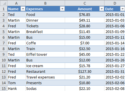
Everything is calculated automatically, the only thing you need to enter is the expenses each person has, see Excel Table in the image above. The date and Expenses columns are not really needed for the calculations.

The formulas in cell G3:H3, and I3 calculates how much each person needs to pay and to who to split expenses evenly based on the amounts in the Excel Table.

Excel 365 dynamic array formula in cell G3:

Excel 365 dynamic array formula in cell H3:

Excel 365 dynamic array formula in cell I3:

The formulas above contain Excel 365 functions and work only in Excel 365, they use values from columns K to M, see image below.

Excel 365 dynamic array formula in cell K3:

Formula in cell L3:

Excel 365 dynamic array formula in cell M3:

Explaining the formula in cell G3

This formula calculates which names will have to pay.

Step 1 - Sum amounts based on conditions

The SUMIF function sums numerical values based on a condition.

Function syntax: SUMIF(range, criteria, [sum_range])

SUMIF($G$2:G2, $K$3#, $H$2:H2) returns {0; 0; 0; 0; 0}.

Step 2 - Add values

The plus sign lets you add numbers in an Excel formula.

$M$3#+SUMIF($G$2:G2, $K$3#, $H$2:H2) returns {39.453; 3... ; -61.197}

Step 3 - Check if sums are lower than 0 (zero)

The less than sign lets you check if a number is smaller than another number, the reuslt is a boolean value TRUE or FALSE.

($M$3#+SUMIF($G$2:G2, $K$3#, $H$2:H2))<0 returns {FALSE;FALSE;TRUE;FALSE;TRUE}.

Step 4 - Count numbers in the spilled formula

The COUNT function counts all numerical values in an argument.

Function syntax: COUNT(value1, [value2], ...)

COUNT($M$3#) returns 5.

Step 5 - Create a sequence from 1 to n

The SEQUENCE function creates a list of sequential numbers.

Function syntax: SEQUENCE(rows, [columns], [start], [step])

SEQUENCE(COUNT($M$3#)) returns {1; 2; 3; 4; 5}.

Step 6 - Replace numbers below zero with the corresponding number in the sequence array

The IF function returns one value if the logical test is TRUE and another value if the logical test is FALSE.

Function syntax: IF(logical_test, [value_if_true], [value_if_false])

IF(($M$3#+SUMIF($G$2:G2, $K$3#, $H$2:H2))<0, SEQUENCE(COUNT($M$3#)), "") returns {""; ""; 3; ""; 5}.

Step 7 - Extract the smallest number in the array

The SMALL function returns the k-th smallest value from a group of numbers.

Function syntax: SMALL(array, k)

SMALL(IF(($M$3#+SUMIF($G$2:G2, $K$3#, $H$2:H2))<0, SEQUENCE(COUNT($M$3#)), ""), 1) returns 3.

Step 8 - Get value from the spilled formula in cell $K$3#

The INDEX function returns a value or reference from a cell range or array, you specify which value based on a row and column number.

Function syntax: INDEX(array, [row_num], [column_num])

INDEX($K$3#, SMALL(IF(($M$3#+SUMIF($G$2:G2, $K$3#, $H$2:H2))<0, SEQUENCE(COUNT($M$3#)), ""), 1)) returns "Fred".

Step 9 - Remove possible errors

The IFERROR function if the value argument returns an error, the value_if_error argument is used. If the value argument does NOT return an error, the IFERROR function returns the value argument.

Function syntax: IFERROR(value, value_if_error)

IFERROR(INDEX($K$3#, SMALL(IF(($M$3#+SUMIF($G$2:G2, $K$3#, $H$2:H2))<0, SEQUENCE(COUNT($M$3#)), ""), 1)), "") returns "Fred".

Explaining the formula in cell H3

This formula calculates the amount to pay.

Step 1 - Sum based on a condition

The SUMIF function sums numerical values based on a condition.

Function syntax: SUMIF(range, criteria, [sum_range])

$G$2:G2 and $H$2:H2 are cell references containing both a relative and absolute part indicated by the $ dollar signs. This makes them grow when the formula cell is copied to the cells below.

$K$3# is a cell reference to cell K3, however, the # (hashtag) makes it reference all spilled values in the Excel 365 dynamic array formula located in cell K3.

SUMIF($G$2:G2,$K$3#,$H$2:H2) returns {0;0;0;0;0}.

Step 2 - Sum based on a condition

The SUMIF function sums numerical values based on a condition.

Function syntax: SUMIF(range, criteria, [sum_range])

SUMIF($I$2:I2,$K$3#,$H$2:H2) returns {0;0;0;0;0}.

Step 3 - Subtract arrays

The minus character lets you subtract numbers in an Excel formula.

SUMIF($G$2:G2,$K$3#,$H$2:H2)-SUMIF($I$2:I2,$K$3#,$H$2:H2) returns {0;0;0;0;0}

Step 4 - Compare

The equal sign lets you compare values in an Excel formula. The result is a boolean value TRUE or FALSE.

$K$3#=G3 returns {FALSE;FALSE;... ;FALSE}.

Step 5 - Filter values

The FILTER function extracts values/rows based on a condition or criteria.

Function syntax: FILTER(array, include, [if_empty])

FILTER($M$3#+SUMIF($G$2:G2,$K$3#,$H$2:H2)-SUMIF($I$2:I2,$K$3#,$H$2:H2),$K$3#=G3) returns -30.822

Step 6 - Filter values

The FILTER function extracts values/rows based on a condition or criteria.

Function syntax: FILTER(array, include, [if_empty])

FILTER($M$3#+SUMIF($G$2:G2,$K$3#,$H$2:H2)-SUMIF($I$2:I2,$K$3#,$H$2:H2),$K$3#=I3) returns 39.453

Step 7 - Remove the negative sign

The ABS function converts negative numbers to positive numbers.

Function syntax: ABS(number)

ABS(FILTER($M$3#+SUMIF($G$2:G2,$K$3#,$H$2:H2)-SUMIF($I$2:I2,$K$3#,$H$2:H2),$K$3#=G3)) returns 30.822

Step 8 - Remove the negative sign

The ABS function converts negative numbers to positive numbers.

Function syntax: ABS(number)

ABS(FILTER($M$3#+SUMIF($G$2:G2,$K$3#,$H$2:H2)-SUMIF($I$2:I2,$K$3#,$H$2:H2),$K$3#=I3)) returns 39.453

Step 9 - Get the smallest number

The MIN function returns the smallest number in a cell range.

Function syntax: MIN(number1, [number2], ...)

MIN(ABS(FILTER($M$3#+SUMIF($G$2:G2,$K$3#,$H$2:H2)-SUMIF($I$2:I2,$K$3#,$H$2:H2),$K$3#=G3)),ABS(FILTER($M$3#+SUMIF($G$2:G2,$K$3#,$H$2:H2)-SUMIF($I$2:I2,$K$3#,$H$2:H2),$K$3#=I3)))

returns 30.822

Step 10 - Remove error values

The IFERROR function if the value argument returns an error, the value_if_error argument is used. If the value argument does NOT return an error, the IFERROR function returns the value argument.

Function syntax: IFERROR(value, value_if_error)

IFERROR(MIN(ABS(FILTER($M$3#+SUMIF($G$2:G2,$K$3#,$H$2:H2)-SUMIF($I$2:I2,$K$3#,$H$2:H2),$K$3#=G3)),ABS(FILTER($M$3#+SUMIF($G$2:G2,$K$3#,$H$2:H2)-SUMIF($I$2:I2,$K$3#,$H$2:H2),$K$3#=I3))),"")

returns 30.822

Step 11 - Shorten the formula

The LET function lets you name intermediate calculation results which can shorten formulas considerably and improve performance.

Function syntax: LET(name1, name_value1, calculation_or_name2, [name_value2, calculation_or_name3...])

IFERROR(MIN(ABS(FILTER($M$3#+SUMIF($G$2:G2,$K$3#,$H$2:H2)-SUMIF($I$2:I2,$K$3#,$H$2:H2),$K$3#=G3)),ABS(FILTER($M$3#+SUMIF($G$2:G2,$K$3#,$H$2:H2)-SUMIF($I$2:I2,$K$3#,$H$2:H2),$K$3#=I3))),"")

w - $H$2:H2,z,$K$3#

x - SUMIF($G$2:G2,z,w)

y - SUMIF($I$2:I2,z,w)

LET(w,$H$2:H2,z,$K$3#,x,SUMIF($G$2:G2,z,w),y,SUMIF($I$2:I2,z,w),IFERROR(MIN(ABS(FILTER($M$3#+x-y,z=G3)),ABS(FILTER($M$3#+x-y,z=I3))),""))

Explaining the formula in cell I3

This formula calculates who will receive the amount. The calculation is almost identical to the one in cell G3 except for steps 1 and 8.

Step 1 - Sum amounts based on conditions

The SUMIF function sums numerical values based on a condition.

Function syntax: SUMIF(range, criteria, [sum_range])

SUMIF($I$2:I2, $K$3#, $H$2:H2) returns {0; 0; 0; 0; 0}.

Step 8 - Get value from the spilled formula in cell $K$3#

The INDEX function returns a value or reference from a cell range or array, you specify which value based on a row and column number.

Function syntax: INDEX(array, [row_num], [column_num])

INDEX($K$3#, SMALL(IF(($M$3#+SUMIF($G$2:G2, $K$3#, $H$2:H2))<0, SEQUENCE(COUNT($M$3#)), ""), 1)) returns "Fred".

Explaining the formula in cell K3

This formula returns a list of unique distinct names, meaning no repeating names.

Step 1 - Create a structured reference to column Name in Table13

The easiest way to create this cell reference is to double-press with left mouse button on cell K3, type =, then select column Name in Excel Table Table13. Excel now creates the cell reference automatically for you.

Why use an Excel Table? The cell reference doesn't change when you add or remove values, you don't have to adjust the cell reference at all like regular cell references. A cell reference to an Excel table is called a structured reference.

Table13[Name]

Step 2 - List unique distinct values

The UNIQUE function returns a unique or unique distinct list.

Function syntax: UNIQUE(array,[by_col],[exactly_once])

UNIQUE(Table13[Name]) returns {"Ted"; "Martin"; "Fred"; "Greg"; "Alice"}.

Explaining the formula in cell L3

This formula calculates the total each person has spent.

Step 1 - Populate arguments

The SUMIF function sums numerical values based on a condition.

Function syntax: SUMIF(range, criteria, [sum_range])

range - Table13[Name]

criteria - K3#

[sum_range] - Table13[Amount]

Step 2 - Evaluate SUMIF function

SUMIF(Table13[Name], K3#,Table13[Amount]) returns {121.85; 120.06; 51.575; 97.3; 21.2}

Explaining the formula in cell M3

This formula calculates the amount to be paid or received, a negative value meaning pay and a positive value meaning receive.

Step 1 - List unique distinct values

The UNIQUE function returns a unique or unique distinct list.

Function syntax: UNIQUE(array,[by_col],[exactly_once])

UNIQUE(Table13[Name]) returns {"Ted"; "Martin"; "Fred"; "Greg"; "Alice"}.

Step 2 - Count non-empty values

The COUNTA function counts the non-empty or non-blank cells in a cell range.

Function syntax: COUNTA(value1, [value2], ...)

COUNTA(UNIQUE(Table13[Name]) returns 5.

Step 3 - Add numbers and return a total

The SUM function allows you to add numerical values, the function returns the sum in the cell it is entered in. The SUM function is cleverly designed to ignore text and boolean values, adding only numbers.

Function syntax: SUM(number1, [number2], ...)

SUM(Table13[Amount]) returns 411.985

Step 4 - Divide the sum with unique distinct count

The division sign lets you perform a division in an Excel formula.

SUM(Table13[Amount])/COUNTA(UNIQUE(Table13[Name])) returns 82.397

Step 5 - Subtract totals in column L with the quotient

The minus sign calculates a difference between two numbers in an Excel formula.

L3#-SUM(Table13[Amount])/COUNTA(UNIQUE(Table13[Name])) returns {39.453; 37.663; -30.822; 14.903; -61.197}.

Get the Excel file

Split-expensesv3.xlsx

Back to top

2. How to split expenses evenly (VBA  Macro)

This workbook lets you split expenses evenly with other people. Type name, expense, and amount in the Excel table on sheet 'Expenses'.

Excel returns amounts to be paid and individuals involved. This is not the macro you are looking for if you want to calculate the smallest number of transactions possible.

How calculation sheet works

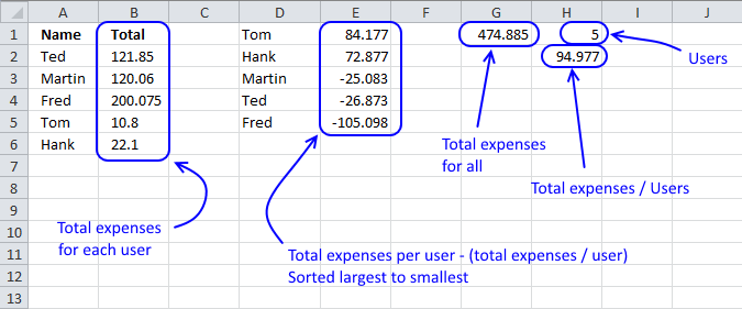
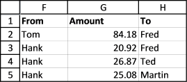
The vba macro uses the values in cell range D1:E5 and calculates transactions so all sums even out.

For example, Tom pays Fred $84.177 and his sum is 84.177 - 84.177 = 0. Hank pays Fred $20.92, Ted $26.87, Martin $25.08 and his sum is 72.88 - 20.92 - 26.87 - 25.08 = 0.

Those were the necessary transactions to even out all user sums to zero. The remaining sums are now all 0, Martin's sum is -25.08 + 25.08 = 0, Ted -26.87 + 26.87 = 0 and Fred -105.098 + 84.177 + 20.92 = 0.

How I made this workbook

There are two sheets in this workbook, 'Expenses' and 'Calculation'. Here are the formulas on 'Calculation' sheet.

Unique distinct names in column A:

Want to know more about this array formula?
Read this post: How to extract a unique distinct list from a column

Sum values for each unique name in column B:

Count unique names in cell H1:

Sum amounts in cell G1:

VBA macro

'Name macro
Sub SplitExp()

'Dimension variables and declare data types
Dim r As Single, d As Single, e As Single, Lrow As Single

'Disable screen refresh
Application.ScreenUpdating = False

'With ... End With statement
With Worksheets("Calculation")

'Save value in cell H1 to variable r
r = .Range("H1")

'Clear everything in columns D to E
.Columns("D:E").Clear

'Clear cell range F2:H100 in worksheet Expenses
Worksheets("Expenses").Range("F2:H100").Clear

'Save values from cell range A2:Br+1 to cell range D1:Er based on variable r
.Range("D" & 1 & ":E" & r) = .Range("A" & 2 & ":B" & r + 1).Value

'For ... Next statement
For d = 1 To r
.Range("E" & d) = (.Range("G1") / r) - .Range("E" & d)
Next d
.Columns("D:E").Sort key1:=.Range("E1"), order1:=xlDescending, Header:=xlNo
For d = 1 To r
For e = r To 1 Step -1
Lrow = Worksheets("Expenses").Range("F" & Rows.Count).End(xlUp).Row + 1
If Round(.Range("E" & d), 2) <> 0 And Round(.Range("E" & e), 2) <> 0 Then
If Application.Min(Abs(.Range("E" & d)), Abs(.Range("E" & e))) = Abs(.Range("E" & d)) Then
Worksheets("Expenses").Range("F" & Lrow & ":H" & Lrow) = Array(.Range("D" & d), Round(Abs(.Range("E" & d)), 2), .Range("D" & e))
.Range("E" & e) = .Range("E" & e) + .Range("E" & d)
.Range("E" & d) = 0
Else
Worksheets("Expenses").Range("F" & Lrow & ":H" & Lrow) = Array(.Range("D" & d), Round(Abs(.Range("E" & e)), 2), .Range("D" & e))
.Range("E" & d) = .Range("E" & e) + .Range("E" & d)
.Range("E" & e) = 0
End If
End If
Next e
Next d
End With
Application.ScreenUpdating = True
End Sub

Event code, sheet 'Calculation'

Private Sub Worksheet_Calculate()

Call SplitExp

End Sub

Back to top

Get the Excel file

Split-expenses-in-excel1.xlsm

Back to top

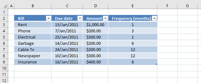
5. Bill reminder

Answer:

Sheet Bills

Sheet Reminder

Array formula in cell B1 sheet Reminder:

How to create an array formula

1. Copy (Ctrl + c) and paste (Ctrl + v) array formula into formula bar.
2. Press and hold Ctrl + Shift.
3. Press Enter once.
4. Release all keys.

How to create an Excel defined Table

I am using an Excel defined Table because a cell reference to an Excel defined table adjusts automatically if you add or remove records.

1. Select a cell in the data set sheet Reminder.
2. Press CTRL + T.
3. Press with left mouse button on checkbox if your data set has headers.
   
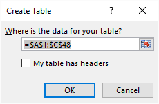
4. Press with left mouse button on OK button.

Explaining array formula in cell B7

The remaining array formulas in cell C7 and D7 are similar to the one in cell B7, they extract a different part of the Excel defined Table.

Step 1

The MONTH function returns a number representing a month based on an Excel date. 1= Jan, 2 = Feb, 3 = March ... 12 = Dec.

MONTH($C$2)=(MONTH(Table1[Due date])+(COLUMN($A$1:$L$1)-1)*Table1[Frequency (months)])

becomes

4=(MONTH(Table1[Due date])+(COLUMN($A$1:$L$1)-1)*Table1[Frequency (months)])

becomes

4={1;1;1;1;1;1;1}+(COLUMN($A$1:$L$1)-1)*Table1[Frequency (months)])

becomes

4={1;1;1;1;1;1;1}+({1,2,3,4,5,6,7,8,9,10,11,12}-1)*Table1[Frequency (months)])

becomes

4={1;1;1;1;1;1;1}+({0, 1, 2, 3, 4, 5, 6, 7, 8, 9, 10, 11})*Table1[Frequency (months)])

becomes

4={1;1;1;1;1;1;1}+({0, 1, 2, 3, 4, 5, 6, 7, 8, 9, 10, 11})*{1;3;1;6;12;12;6})

becomes

4={1;1;1;1;1;1;1}+{0, 1, 2, ... , 66}

becomes

4={1, 2,... , 67}

and returns

{FALSE, ... , FALSE}

Step 2

The DAY function returns the day of an Excel date.

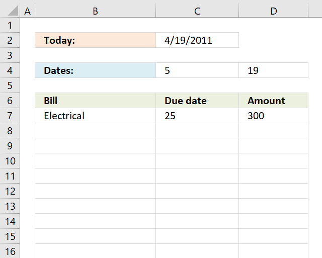
(DAY($C$2)<$C$4)*(DAY(Table1[Due date])>=$D$4)

becomes

(19<5)*({15;7;25;14;24;10;16}>=19)

becomes

FALSE*{FALSE; FALSE; TRUE; FALSE; TRUE; FALSE; FALSE}

and returns {0; 0; 0; 0; 0; 0; 0}

Step 3

(DAY($C$2)>=$C$4)*(DAY($C$2)<$D$4)*(DAY(Table1[Due date])>=$C$4)*(DAY(Table1[Due date])<$D$4)

becomes

(19>=5)*(19<19)*({15;7;25;14;24;10;16}>=5)*({15;7;25;14;24;10;16}<19)

becomes

TRUE*FALSE*{1;1;0;1;0;1;1}

and returns

{0; 0; 0; 0; 0; 0; 0}

Step 4

(DAY($C$2)>=$D$4)*(DAY(Table1[Due date])>=$D$4)

becomes

(19>=19)*({15;7;25;14;24;10;16}>=19)

becomes

TRUE*{FALSE; FALSE; TRUE; FALSE; TRUE; FALSE; FALSE}

and returns

{0; 0; 1; 0; 1; 0; 0}

Step 5 - Add/Multiply arrays

AND logic - Multiply arrays

OR logic - Add arrays

(MONTH($C$2)=(MONTH(Table1[Due date])+(COLUMN($A$1:$L$1)-1)*Table1[Frequency (months)]))*((DAY($C$2)<$C$4)*(DAY(Table1[Due date])>=$D$4)+(DAY($C$2)>=$C$4)*(DAY($C$2)<$D$4)*(DAY(Table1[Due date])>=$C$4)*(DAY(Table1[Due date])<$D$4)+(DAY($C$2)>=$D$4)*(DAY(Table1[Due date])>=$D$4))

becomes

{FALSE,... , FALSE}*({0; 0; 0; 0; 0; 0; 0}+{0; 0; 0; 0; 0; 0; 0}+{0; 0; 1; 0; 1; 0; 0})

becomes

{FALSE, ... , FALSE}*{0;0;1;0;1;0;0}

and returns

{0, ... , 1, ... , 0}

Step 6 - Convert TRUE (1) to corresponding row number

The IF function has three arguments, the first one must be a logical expression. If the expression evaluates to TRUE then one thing happens (argument 2) and if FALSE another thing happens (argument 3).

IF((MONTH($C$2)=(MONTH(Table1[Due date])+(COLUMN($A$1:$L$1)-1)*Table1[Frequency (months)]))*((DAY($C$2)<$C$4)*(DAY(Table1[Due date])>=$D$4)+(DAY($C$2)>=$C$4)*(DAY($C$2)<$D$4)*(DAY(Table1[Due date])>=$C$4)*(DAY(Table1[Due date])<$D$4)+(DAY($C$2)>=$D$4)*(DAY(Table1[Due date])>=$D$4)), ROW(Table1[Due date])-MIN(ROW(Table1[Due date]))+1, "")

returns

{"", ... , 3, ... , ""}

Step 7 - Extract k-th smallest row number in array

The SMALL function returns the k-th smallest value in a cell range or array. SMALL( array, k)

SMALL(IF((MONTH($C$2)=(MONTH(Table1[Due date])+(COLUMN($A$1:$L$1)-1)*Table1[Frequency (months)]))*((DAY($C$2)<$C$4)*(DAY(Table1[Due date])>=$D$4)+(DAY($C$2)>=$C$4)*(DAY($C$2)<$D$4)*(DAY(Table1[Due date])>=$C$4)*(DAY(Table1[Due date])<$D$4)+(DAY($C$2)>=$D$4)*(DAY(Table1[Due date])>=$D$4)), ROW(Table1[Due date])-MIN(ROW(Table1[Due date]))+1, ""), ROW(A1))

becomes

SMALL({"", ... , 3, ... , ""}, ROW(A1))

becomes

SMALL({"", ... , 3, ..., ""}, 1)

and returns 3.

Step 8 - Return value

The INDEX function returns a value based on a row and column number.

INDEX(Table1[Bill], SMALL(IF((MONTH($C$2)=(MONTH(Table1[Due date])+(COLUMN($A$1:$L$1)-1)*Table1[Frequency (months)]))*((DAY($C$2)<$C$4)*(DAY(Table1[Due date])>=$D$4)+(DAY($C$2)>=$C$4)*(DAY($C$2)<$D$4)*(DAY(Table1[Due date])>=$C$4)*(DAY(Table1[Due date])<$D$4)+(DAY($C$2)>=$D$4)*(DAY(Table1[Due date])>=$D$4)), ROW(Table1[Due date])-MIN(ROW(Table1[Due date]))+1, ""), ROW(A1)), 1)

returns "Electrical" in cell B7.

Step 9 - Avoid errors

The IFERROR function returns a blank if formula returns an error.

Array formula in cell C1:

Array formula in cell D1:

Get the Excel file

Bill-reminder-version3.xlsx

Split values category

Split data across multiple sheets – VBA
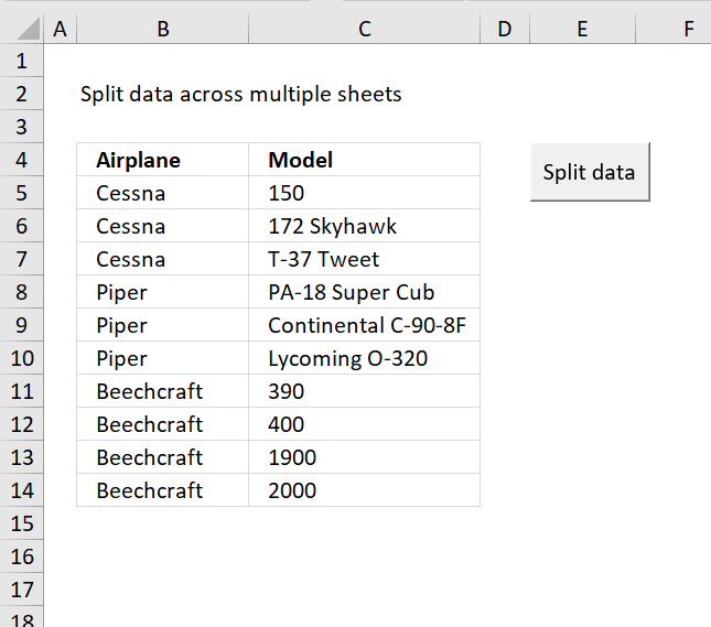
Table of Contents Split data across multiple sheets - VBA Add values to worksheets based on a condition - VBA […]

A Comprehensive Guide to Splitting Text in Excel
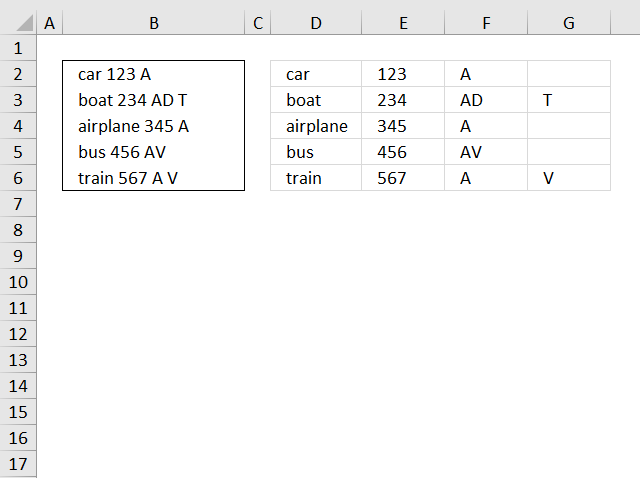
This blog article describes how to split strings in a cell with space as a delimiting character, like Text to […]

Excel categories

Comments (17)