If cell contains text from list
This article demonstrates several techniques to check if a cell contains text based on a list. The first example shows how to check if text in the list is in the cell.
The remaining examples show formulas that check if a cell contains text and also identify which text the cell contains. This article demonstrates different formulas for different Excel versions.
What's on this page
- Check if the cell contains text in the list
- Display matches if cell contains text from list (Excel 2019)
- Display matches if cell contains text from list (Earlier Excel versions)
- Filter delimited values not in list (Excel 365)
- Check if cell contains text in the list and return the corresponding value
- Get Excel *.xlsx file
- If cell equals value
- If cell contains multiple values
- If cell equals value from list
- If cell contains text
1. Check if the cell contains any value in the list
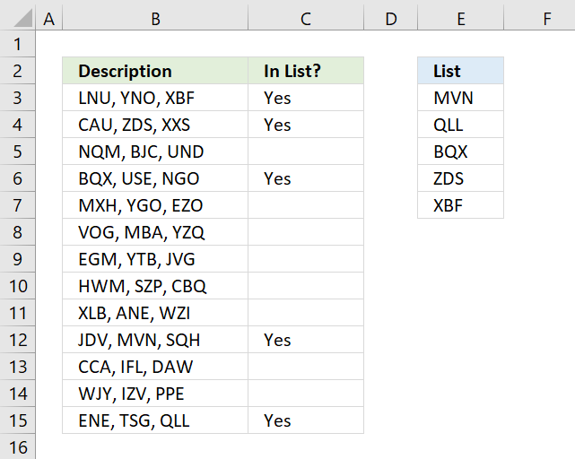
The image above shows an array formula in cell C3 that checks if cell B3 contains at least one of the values in List (E3:E7), it returns "Yes" if any of the values are found in column B and returns nothing if the cell contains none of the values.
For example, cell B3 contains XBF which is found in cell E7. Cell B4 contains text ZDS found in cell E6. Cell C5 contains no values in the list.
You need to enter this formula as an array formula if you are not an Excel 365 subscriber. There is another formula below that doesn't need to be entered as an array formula, however, it is slightly larger and more complicated.
- Type formula in cell C3.
- Press and hold CTRL + SHIFT simultaneously.
- Press Enter once.
- Release all keys.
Excel adds curly brackets to the formula automatically if you successfully entered the array formula. Don't enter the curly brackets yourself.
1.1 Explaining formula in cell C3
Step 1 - Check if the cell contains any of the values in the list
The COUNTIF function lets you count cells based on a condition, however, it also allows you to count cells based on multiple conditions if you use a cell range instead of a cell.
COUNTIF(range, criteria)
The criteria argument utilizes a beginning and ending asterisk in order to match a text string and not the entire cell value, asterisks are one of two wildcard characters that you are allowed to use.
The ampersands concatenate the asterisks to cell range E3:E7.
COUNTIF(B3,"*"&$E$3:$E$7&"*")
returns this array
{0; 0; 0; 0; 1}
which tells us that the last value in the list is found in cell B3.
Step 2 - Return TRUE if at least one value is 1
The OR function returns TRUE if at least one of the values in the array is TRUE, the numerical equivalent to TRUE is 1.
OR({0; 0; 0; 0; 1})
returns TRUE.
Step 3 - Return Yes or nothing
The IF function then returns "Yes" if the logical test evaluates to TRUE and nothing if the logical test returns FALSE.
IF(TRUE, "Yes", "")
returns "Yes" in cell B3.
Regular formula
The following formula is quite similar to the formula above except that it is a regular formula and it has an additional INDEX function.
2. Display matches if the cell contains text from a list

The image above demonstrates a formula that checks if a cell contains a value in the list and then returns that value. If multiple values match then all matching values in the list are displayed.
For example, cell B3 contains "ZDS, YNO, XBF" and cell range E3:E7 has two values that match, "ZDS" and "XBF".
Formula in cell C3:
The TEXTJOIN function is available for Office 2019 and Office 365 subscribers. You will get a #NAME error if your Excel version is missing this function. Office 2019 users may need to enter this formula as an array formula.
The next formula works with most Excel versions.
Array formula in cell C3:
However, it only returns the first match. There is another formula below that returns all matching values, check it out.
2.1 Explaining formula in cell C3
Step 1 - Count cells containing text strings
The COUNTIF function lets you count cells based on a condition, we are going to use multiple conditions. I am going to use asterisks to make the COUNTIF function check for a partial match.
The asterisk is one of two wild card characters that you can use, it matches 0 (zero) to any number of any characters.
COUNTIF(B3, "*"&$E$3:$E$7&"*")
returns {1; 0; 0; 0; 1}.
This array contains as many values as there values in the list, the position of each value in the array matches the position of the value in the list. This means that we can tell from the array that the first value and the last value is found in cell B3.
Step 2 - Return the actual value
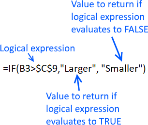
The IF function returns one value if the logical test is TRUE and another value if the logical test is FALSE.
IF(logical_test, [value_if_true], [value_if_false])
This allows us to create an array containing values that exists in cell B3.
IF(COUNTIF(B3, "*"&$E$3:$E$7&"*"), $E$3:$E$7, "")
returns {"";"";"";"ZDS";"XBF"}.
Step 3 - Concatenate values in array
The TEXTJOIN function allows you to combine text strings from multiple cell ranges and also use delimiting characters if you want.
TEXTJOIN(delimiter, ignore_empty, text1, [text2], ...)
TEXTJOIN(", ", TRUE, IF(COUNTIF(B3, "*"&$E$3:$E$7&"*"), $E$3:$E$7, ""))
returns text strings ZDS, XBF.
3. Display matches if cell contains text from a list (Earlier Excel versions)

The image above demonstrates a formula that returns multiple matches if the cell contains values from a list. This array formula works with most Excel versions.
Array formula in cell C3:
Copy cell C3 and paste to cell range C3:E15.
3.1 Explaining formula in cell C3
Step 1 - Identify matching values in cell
The COUNTIF function lets you count cells based on a condition, we are going to use a cell range instead. This will return an array of values.
COUNTIF($B3, "*"&$G$3:$G$7&"*")
returns {0; 0; 0; 1; 1}.
Step 2 - Calculate relative positions of matching values
The IF function returns one value if the logical test is TRUE and another value if the logical test is FALSE.
IF(logical_test, [value_if_true], [value_if_false])
This allows us to create an array containing values representing row numbers.
IF(COUNTIF($B3, "*"&$G$3:$G$7&"*"), MATCH(ROW($G$3:$G$7), ROW($G$3:$G$7)), "")
returns {""; ""; ""; 4; 5}.
Step 3 - Extract the k-th smallest number
I am going to use the SMALL function to be able to extract one value in each cell in the next step.
SMALL(array, k)
SMALL(IF(COUNTIF($B3, "*"&$G$3:$G$7&"*"), MATCH(ROW($G$3:$G$7), ROW($G$3:$G$7)), ""), COLUMNS($A$1:A1)))
returns 4.
Step 4 - Return value based on row number
The INDEX function returns a value from a cell range or array, you specify which value based on a row and column number. Both the [row_num] and [column_num] are optional.
INDEX(array, [row_num], [column_num])
INDEX($G$3:$G$7, SMALL(IF(COUNTIF($B3, "*"&$G$3:$G$7&"*"), MATCH(ROW($G$3:$G$7), ROW($G$3:$G$7)), ""), COLUMNS($A$1:A1)))
returns "ZDS" in cell C3.
Step 5 - Remove error values
The IFERROR function lets you catch most errors in Excel formulas except #SPILL! errors. Be careful when using the IFERROR function, it may make it much harder spotting formula errors.
IFERROR(value, value_if_error)
There are two arguments in the IFERROR function. The value argument is returned if it is not evaluating to an error. The value_if_error argument is returned if the value argument returns an error.
IFERROR(INDEX($G$3:$G$7, SMALL(IF(COUNTIF($B3, "*"&$G$3:$G$7&"*"), MATCH(ROW($G$3:$G$7), ROW($G$3:$G$7)), ""), COLUMNS($A$1:A1))), "")
4. Filter delimited values not in the list (Excel 365)

The formula in cell C3 lists values in cell B3 that are not in the List specified in cell range E3:E7. The formula returns #CALC! error if all values are in the list, see cell C14 as an example.
Excel 365 dynamic array formula in cell C3:
4.1 Explaining formula
Step 1 - Split values with a delimiting character
The TEXTSPLIT function splits a string into an array based on delimiting values.
Function syntax: TEXTSPLIT(Input_Text, col_delimiter, [row_delimiter], [Ignore_Empty])
TEXTSPLIT(B3,,",")
returns
{"ZDS"; " VTO"; " XBF"}
Step 2 - Remove leading and trailing spaces
The TRIM function deletes all blanks or space characters except single blanks between words in a cell value.
Function syntax: TRIM(text)
TRIM(TEXTSPLIT(B3,,","))
returns
{"ZDS"; "VTO"; "XBF"}
Step 3 - Check if values are in list
The COUNTIF function calculates the number of cells that is equal to a condition.
Function syntax: COUNTIF(range, criteria)
COUNTIF($E$3:$E$7,TRIM(TEXTSPLIT(B3,,",")))
returns
{1; 0; 1}
These numbers indicate if a value is found in the list, zero means not in the list and 1 or higher means that the value is in the list at least once.
The number's position corresponds to the position of the values. {1; 0; 1} - {"ZDS"; "VTO"; "XBF"} meaning "ZDS" and "XBF" are in the list and "VTO" not.
Step 4 - Not
The NOT function returns the boolean opposite to the given argument.
Function syntax: NOT(logical)
NOT(COUNTIF($E$3:$E$7,TRIM(TEXTSPLIT(B3,,","))))
returns
{FALSE; TRUE; FALSE}.
0 (zero) is equivalent to FALSE. The boolean opposite is TRUE.
Any other number than 0 (zero) is equivalent to TRUE. The boolean opposite is FALSE.
Step 5 - Filter
The FILTER function extracts values/rows based on a condition or criteria.
Function syntax: FILTER(array, include, [if_empty])
FILTER(TRIM(TEXTSPLIT(B3,,",")),NOT(COUNTIF($E$3:$E$7,TRIM(TEXTSPLIT(B3,,",")))))
returns
"VTO".
Step 6 - Join
The TEXTJOIN function combines text strings from multiple cell ranges.
Function syntax: TEXTJOIN(delimiter, ignore_empty, text1, [text2], ...)
TEXTJOIN(", ",TRUE,FILTER(TRIM(TEXTSPLIT(B3,,",")),NOT(COUNTIF($E$3:$E$7,TRIM(TEXTSPLIT(B3,,","))))))
returns "VTO".
Step 7 - Shorten the formula
The LET function lets you name intermediate calculation results which can shorten formulas considerably and improve performance.
Function syntax: LET(name1, name_value1, calculation_or_name2, [name_value2, calculation_or_name3...])
TEXTJOIN(", ",TRUE,FILTER(TRIM(TEXTSPLIT(B3,,",")),NOT(COUNTIF($E$3:$E$7,TRIM(TEXTSPLIT(B3,,","))))))
TRIM(TEXTSPLIT(B3,,",")) is repeated once.
z - TRIM(TEXTSPLIT(B3,,","))
LET(z,TRIM(TEXTSPLIT(B3,,",")),TEXTJOIN(", ",TRUE,FILTER(z,NOT(COUNTIF($E$3:$E$7,z)))))
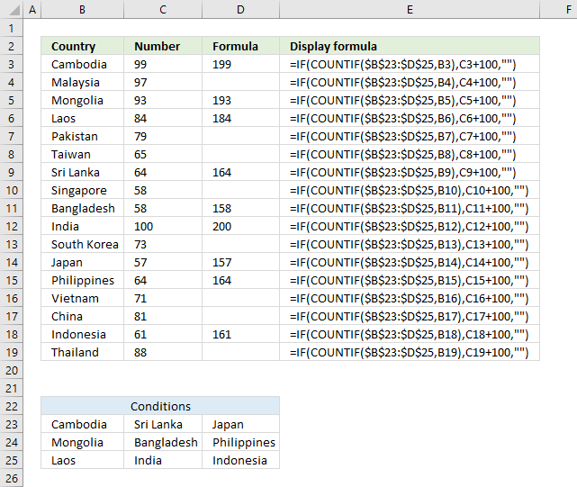
5. Check if cell contains value in the list and return the corresponding value

The following formula checks cell range e3:e7 but returns the value of the corresponding cell in F3:F7.
Formula in cell C3:
For example, cell B3 contains "ZDS, YNO, XBF". It contains two value in cell range E3:E7 namely "ZDS" and "XBF", the corresponding values in cell range F3:F7 are 4 and 9.
Links
COUNTIF function - Microsoft
INDEX function - Microsoft
TEXTJOIN function - Microsoft
7. If cell equals value
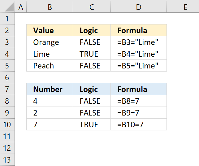
The easiest way to check if a cell has a value is, in my opinion, to use the equal sign to compare the cell value with the value you are looking for.
The equal sign is a logical operator that turns the formula a logical expression and returns a boolean value, TRUE or FALSE.
Formula in cell C3:
Use double quotation marks before and after the text value in order to do the comparison. B3 is a cell reference to a specific cell at the intersection of column B and row 3.
Copy cell C3 and paste to cells below and the cell reference changes in each cell. B3 is, therefore, a relative cell reference.
If you forget the double quotation marks Excel will evaluate your text value as a built-in function or a user-defined function. If such function can't be found Excel returns #NAME? error.
Formula in cell D8:
Don't use double quotation marks with numbers, if you do Excel will evaluate your number as a text value and the comparison will never return TRUE.
Example,
returns FALSE even though cell B10 has number 7.
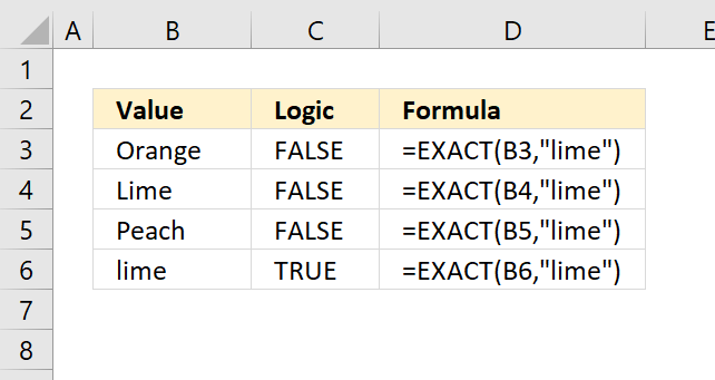
The comparison made by the equal sign is, however, not case-sensitive. Use the EXACT function to perform a case-sensitive comparison, see picture above.
A formula like this one has one of the values hardcoded into the formula:
If you want to compare another value you must change each formula in every cell which is not at all efficient.
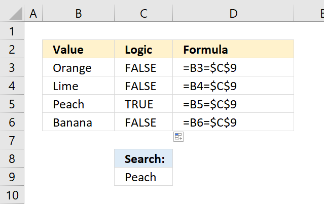
The picture above shows a formula that compares two cell values, however, one of the cell references are locked to cell C9.
How did I enter this formula?
- Double press with left mouse button on cell C3 with left mouse button.
- Type =B3=C9
- Press function key F4 to automatically change C9 to $C$9.
- Press Enter
- Copy cell C3
- Paste to cells below.
If you now examine the formula you will see that the first cell reference B3 in the formula changes in each cell.
This happens with relative cell reference whereas an absolute cell reference doesn't change.
Having cell references in your formulas allows you to quickly change a value without adjusting the cell formulas at all.
Try it yourself, change the value in cell C9 to Banana and check column C for changes. Cell C6 is now TRUE and C5 is FALSE.
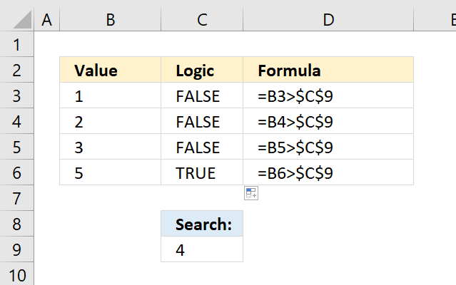
The equal sign (=) is one out of 3 different logical operators, the picture above shows you the greater than sign (>).
You can combine these three logical operators to perform different logical expressions, see table below.
| Logical operator | Description | Example |
| < | less than | B3<$C$9 |
| > | greater than | B3>$C$9 |
| <= | less than or equal to | B3<=$C$9 |
| >= | greater than or equal to | B3>=$C$9 |
| = | equal to | B3=$C$9 |
| <> | not equal to | B3<>$C$9 |
The formula in column C returns TRUE if the value in column B is larger than 4.
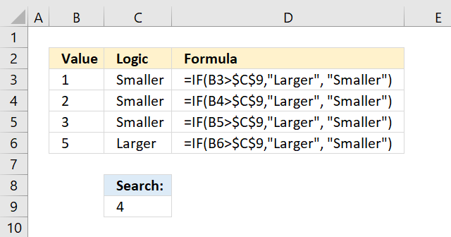
Now you know what a logical expression is which is an essential part of an IF function.
Get Excel *.xlsx file
8. If cell contains multiple values
This section demonstrates formulas that perform a partial match for a given cell using multiple strings specified in cells F2 and F3.
Table of Contents
- Find cells containing all conditions
- Find cells containing all conditions (Excel 365)
- Find cells containing at least one condition
- Get Excel *.xlsx file
8.1. Find cells containing all conditions
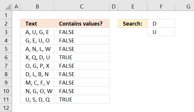
The array formula in cell C3 checks if the value in cell B3 contains all conditions specified in cells F2:F3, it returns a boolean value TRUE or FALSE.
Both conditions must be found in cell C3 in order to return TRUE. For example, cell B4 contains one of the two conditions, however, the formula returns FALSE in cell C4.
8.1.1 How to enter an array formula

To enter an array formula, type the formula in a cell then press and hold CTRL + SHIFT simultaneously, now press Enter once. Release all keys.
The formula bar now shows the formula with a beginning and ending curly bracket telling you that you entered the formula successfully. Don't enter the curly brackets yourself.
8.1.2 Explaining formula in cell C3
Step 1 - Find cells containing at least one condition
The SEARCH function returns the character position of a substring in a text string, it returns an error if not found.
SEARCH(find_text,within_text, [start_num])
SEARCH($F$2:$F$3,B3)
becomes
SEARCH({"D";"U"},"A, U, G, E")
and returns {#VALUE!;4}.
Step 2 - Count numbers in array
The COUNT function counts the number of values that contain a number, it conveniently also ignores errors.
COUNT(value1, [value2], ...)
COUNT(SEARCH($F$2:$F$3,B3))
becomes
COUNT({#VALUE!; 4})
and returns 1. Only one value in the array is a number.
Step 2 - Count numbers in the array
Lastly, the equal sign compares the output with number 2. There are two conditions specified in cells F2 and F3, this is why the count is compared to two.
COUNT(SEARCH($F$2:$F$3,B3))=2
becomes
1=2
and returns FALSE in cell C3.
8.2. Find cells containing at least one condition

If you want the formula to return TRUE if at least one value is found change the array formula to:
The formula above is almost identical to the formula in section 1, however, there are two comparison operators in this formula instead of one.
The equal sign and the larger than sign combined lets you check if a value is equal to or larger than a given condition. Read section 1.2 for a more detailed explanation.
The possibilities are endless here if you want the formula to return TRUE if at least 2 out of 3 values are found, change the formula to:
8.3. Find cells containing all conditions (regular formula)

This formula is slightly larger but has the advantage of being a regular formula, no need to enter the formula as an array formula.
Explaining formula in cell C3
Step 1 - Append asterisks to each condition
The ampersand character lets you concatenate strings in an Excel formula. The asterisk character is a wildcard character that matches 0 (zero) to any length of characters.
The part shown below appends asterisks to the start and end of each string in cells F2 and F3.
"*"&$F$2:$F$3&"*"
returns
{"*D*"; "*U*"}.
Step 2 - Count values using partial match
The COUNTIF function calculates the number of cells that is equal to a condition.
COUNTIF(range, criteria)
COUNTIF(B3,"*"&$F$2:$F$3&"*")
returns {0; 1}.
Step 3 - Multiply by 1
This step is required to convert the array formula to a regular formula, this step is not needed if you are using Excel 365.
COUNTIF(B3,"*"&$F$2:$F$3&"*")*1
becomes
{0; 1}*1
and returns {0; 1}.
Step 4 - Add numbers in array and return a total
The SUMPRODUCT function calculates the product of corresponding values and then returns the sum of each multiplication.
SUMPRODUCT(array1, [array2], ...)
SUMPRODUCT(COUNTIF(B3,"*"&$F$2:$F$3&"*")*1)
becomes
SUMPRODUCT({0; 1})
and returns 1.
Step 5 - Compare the result to two
The equal sign compare the result to two, this makes the formula return TRUE if both string are found. Change this value if you have more or fewer conditions.
SUMPRODUCT(COUNTIF(B3,"*"&$F$2:$F$3&"*")*1)=2
becomes
1=2
and returns FALSE in cell C3.
8.4 Get Excel *.xlsx file
If cell contains multiple values.xlsx
9. If cell equals value from list
This section demonstrates formulas that check if a cell value is equal to any value in a given list.
Table of Contents
- If cell equals value from list - regular formula
- If cell equals value from list - array formula
- Alternative regular formula
- If cell equals value from list - case sensitive
- Get Excel *.xlsx file
9.1. If cell equals value from list - regular formula

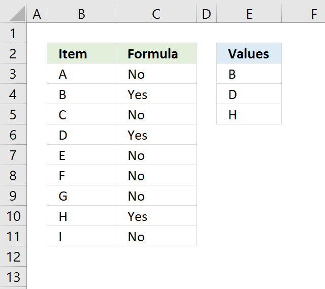
This example demonstrates a formula that returns "Yes" if the adjacent cell on the same row is equal to at least one of the values in cell range E3:E5. "No" is returned if none of the values is equal to the adjacent value in column B.
Formula in cell C3:
For example, cell B3 contains value "A". The formula in cell C3 returns "No" because none of the values in cell range E3:E5 is equal to "A".
Explaining formula in cell C3
Step 1 - Count cells based on condition
The COUNTIF function counts how many values in E3:E5 match cell B3, it returns 0 (zero) since "A" is not found in E3:A5.
COUNTIF(range, criteria)
COUNTIF($E$3:$E$5,B3)
returns 0 (zero).
Step 2 - Count cells based on condition
The IF function then returns "YES" if the logical expression is 1 or more, "No" if the logical expression returns 0 (zero).
IF(logical_test, [value_if_true], [value_if_false])
IF(COUNTIF($E$3:$E$5,B3),"Yes","No")
becomes
IF(0,"Yes","No") and returns "No" in cell C3.
9.2. If cell equals value from list - array formula

I recommend using the regular formula above, this array formula checks if cell B3 is equal to any of the values in E3:E5, the IF function returns Yes if one of the values is a match and No if none of the values match.
Excel 365 users can enter this formula as a regular formula.
9.2.1 How to enter an array formula
To enter an array formula, type the formula in a cell and then press and hold CTRL + SHIFT simultaneously, now press Enter once. Release all keys.
The formula bar now shows the formula enclosed with curly brackets telling you that you entered the formula successfully. Don't enter the curly brackets yourself.
9.2.2 Explaining formula in cell C3
Step 1 - Compare values
The equal sign compares the value in cell B3 with each value in cell range E3:E5.
B3=$E$3:$E$5
returns {FALSE; FALSE; FALSE}. If the cell matches a value in E3:E5 it returns TRUE, if not FALSE. In this case, all logical expressions return FALSE.
Step 2 - Evaluate OR function
The OR function returns TRUE if at least one argument is TRUE.
OR(logical1, [logical2])
OR(B3=$E$3:$E$5)
becomes
OR({FALSE; FALSE; FALSE})
and returns FALSE. The OR function returns FALSE since all arguments are FALSE.
Step 3 - Evaluate IF function
The IF function returns "YES" if the logical expression is TRUE, "No" if the logical expression is FALSE.
IF(logical_test, [value_if_true], [value_if_false])
IF(OR(B3=$E$3:$E$5),"Yes","No")
IF(FALSE,"Yes","No")
and returns "No". The IF function then returns No in cell C3.
Alternative regular formula
The INDEX function changes the above formula into a regular formula.
The INDEX and SUMPRODUCT functions have this characteristic, you just have to know when and where to apply them.
Related post
Recommended articles
The image above demonstrates a formula that matches a value to multiple conditions, if the condition is met the formula […]
9.4. If cell equals value from list case sensitive

This example demonstrates a formula that performs a case sensitive comparison between a given value and multiple values in a cell range.
Array formula in cell C3:
For example, cell B4 contains "B" and the formula in cell C4 returns "No" because none of the values in cell range E3:E5 is equal to the value also considering upper and lower letters.
Excel 365 users can enter this formula as a regular formula.
9.4.1 Explaining formula in cell C3
Step 1 - Identify equal values case sensitive
The EXACT function lets you compare values also considering upper and lower cases.
EXACT(text1, text2)
EXACT(B3, $E$3:$E$5)
becomes
EXACT("A", {"b"; "D"; "H"})
and returns
{FALSE; FALSE; FALSE}.
Step 2 - Evaluate OR function
The OR function returns TRUE if at least one argument is TRUE.
OR(logical1, [logical2])
OR(EXACT(B3, $E$3:$E$5))
becomes
OR({FALSE; FALSE; FALSE})
and returns FALSE.
Step 3 - Evaluate IF function
The IF function returns "YES" if the logical expression is TRUE, "No" if the logical expression is FALSE.
IF(logical_test, [value_if_true], [value_if_false])
IF(OR(EXACT(B3, $E$3:$E$5)), "Yes", "No")
becomes
IF(FALSE, "Yes", "No")
and returns "No".
9.5. Get Excel *.xlsx file
If cell equals value from list.xlsx
10. If cell contains text

This section demonstrates different formulas based on if a cell contains a given text.
Formula in cell C3:
The formula shown in the image above in cell C3 returns TRUE or FALSE based on a comparison between cell B3 and cell E3. The equal sign is a logical operator and returns boolean value TRUE or FALSE, it is not case sensitive.
Table of Contents
- If cell contains partial text
- Explaining formula
- If cell contains partial text - hardcoded asterisks
- Alternative function - SEARCH function
- If cell contains text then return value
- If cell contains text then add text in another cell
- If cell contains text then sum
- If cell contains text add 1
- Highlight cell if cell contains text (Link)
- Get Excel file
10.1. If cell contains partial text

The easiest way to check if a cell partially contains a specific text string is, in my opinion, the IF and COUNTIF function combined. The COUNTIF function allows you to count how many times a text string exists in a cell range.
Formula in cell D3:
The asterisk characters let you perform a wildcard match meaning that it matches any sequence of characters. Adding a beginning and ending asterisk to a text string allows you to check if a cell value contains a specific text string.
10.1.1 Explaining formula in cell D3
Step 1 - Check if cell contains text condition
You can't use asterisks with the equal sign to check if a cell contains a given text, however, the COUNTIF function can do that.
The COUNTIF function calculates the number of cells that is equal to a condition.
COUNTIF(range, criteria)
COUNTIF(B3, C3) returns 1.
Step 2 - Evaluate IF function
The IF function returns one value if the logical test is TRUE and another value if the logical test is FALSE.
IF(logical_test, [value_if_true], [value_if_false])
IF(COUNTIF(B3, C3), TRUE, FALSE) becomes IF(1, TRUE, FALSE)
The logical_test argument requires boolean values or their numerical equivalents. FALSE = 0 (zero), TRUE any number except zero.
10.1.2 If cell contains partial text - hardcoded asterisks

Formula in cell D4:
You don't have to add asterisks manually to your cell, you can easily build a formula that adds the asterisks automatically, demonstrated in cell D4. The ampersand & character lets you append the asterisks to the text string you want to use.
Note, if a text string is found twice in the same cell the COUNTIF function only returns 1. It counts cells not text strings.
10.1. Alternative function - SEARCH function
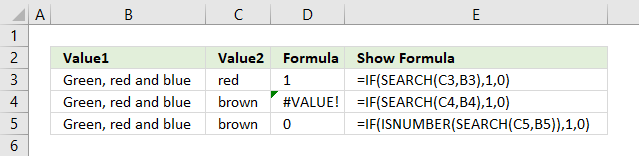
The SEARCH function returns the position of the character at which a specific text string is found. Luckily the IF function accepts any number as TRUE except 0 (zero), however, the SEARCH function returns an error #VALUE! if it can't find the text string.
Formula in cell D5:
To avoid the error value I use the ISNUMBER function that returns TRUE if a number and FALSE if anything else, also formula errors.
10.2. If cell contains text then return value

The formula in cell C3 checks if cell B3 contains the condition specified in cell E3. It returns the value if TRUE and a blank cell if FALSE.
Formula in cell C3:
10.2.1 Explaining formula in cell C3
Step 1 - Concatenate strings
The asterisk is a wildcard character that matches 0 (zero) to any number of characters. The ampersand character concatenates strings in an Excel formula.
"*"&$E$3&"*" becomes "*"&"purple"&"*" and returns "*purple*".
Step 2 - Check if cell contains string
The COUNTIF function calculates the number of cells that is equal to a condition.
COUNTIF(range, criteria)
COUNTIF(B3, "*"&$E$3&"*")
becomes
COUNTIF("Green, red and blue", "*purple*")
and returns 0 (zero). Purple is not found in cell B3.
Step 3 - Return value if TRUE
The IF function returns one value if the logical test is TRUE and another value if the logical test is FALSE.
IF(logical_test, [value_if_true], [value_if_false])
IF(COUNTIF(B3, "*"&$E$3&"*"), B3, "")
becomes
IF(0, B3, "")
and returns "" in cell C3.
10.3. If cell contains text then add text from another cell

The formula in cell C3 checks if cell B3 contains the condition specified in cell E3. It returns the value concatenated with a value on the same row from column if TRUE and a blank cell if FALSE.
Formula in cell C3:
10.3.1 Explaining formula in cell C4
Step 1 - Concatenate strings
The asterisk is a wildcard character that matches 0 (zero) to any number of characters. The ampersand character concatenates strings in an Excel formula.
"*"&$E$3&"*"
becomes
"*"&"purple"&"*"
and returns "*purple*".
Step 2 - Check if cell contains string
The COUNTIF function calculates the number of cells that is equal to a condition.
COUNTIF(range, criteria)
COUNTIF(B4, "*"&$E$3&"*")
becomes
COUNTIF("Black, purple, white", "*purple*")
and returns 1. Purple is found in cell B4.
Step 3 - Return concatenated value if TRUE
The IF function returns one value if the logical test is TRUE and another value if the logical test is FALSE.
IF(logical_test, [value_if_true], [value_if_false])
IF(COUNTIF(B4, "*"&$E$3&"*"), B4&C4, "")
becomes
IF(0, B4&C4, "")
becomes
IF(0, "Black, purple, white"&"#11", "")
and returns "Black, purple, white#11" in cell D4.
10.4. If cell contains text then sum

The formula in cell F3 checks if cells in column B contain the condition specified in cell E3 and sums the corresponding values in column C.
Formula in cell C3:
10.4.1 Explaining formula in cell C4
Step 1 - Search for string
The SEARCH function returns a number representing the position of character at which a specific text string is found reading left to right. It is not a case-sensitive search.
SEARCH(find_text,within_text, [start_num])
SEARCH(E3, B3:B6)
becomes
SEARCH("North", {"North, South"; "South, East"; "West, North, South"; "South, West"})
and returns {1; #VALUE!; 7; #VALUE!}.
Step 2 - Check if value in array is an error
The ISNUMBER function checks if a value is a number, returns TRUE or FALSE.
ISNUMBER(SEARCH(E3, B3:B6))
becomes
ISNUMBER({1; #VALUE!; 7; #VALUE!})
and returns {TRUE; FALSE; TRUE; FALSE}.
Step 3 - Multiply corresponding numbers
The asterisk lets you multiply numbers in an Excel formula. We are multiplying boolean values in this example.
ISNUMBER(SEARCH(E3, B3:B6))*C3:C6
becomes
{TRUE; FALSE; TRUE; FALSE}*{10; 15; 6; 2}
TRUE equals 1 and FALSE equals 0 (zero).
{TRUE; FALSE; TRUE; FALSE}*{10; 15; 6; 2}
and returns {10; 0; 6; 0}.
Step 4 - Sum numbers
The SUM function adds numbers and returns a total.
SUM(ISNUMBER(SEARCH(E3, B3:B6))*C3:C6)
becomes
SUM({10; 0; 6; 0})
and returns 16 in cell F3.
10.5. If cell contains text add 1

The formula in cell C3 counts cells containing the given text string in cell E3.
Formula in cell C3:
10.5.1 Explaining formula in cell C3
Step 1 - Concatenate strings
The asterisk is a wildcard character that matches 0 (zero) to any number of characters. The ampersand character concatenates strings in an Excel formula.
"*"&$E$3&"*"
becomes
"*"&"North"&"*"
and returns "*North*".
Step 2 - Check if cell contains given string
The COUNTIF function calculates the number of cells that is equal to a condition.
COUNTIF(range, criteria)
COUNTIF(B3,"*"&$E$3&"*")
becomes
COUNTIF("North, South", "*North*")
and returns 1.
Step 3 - Calculate count
The MAX function returns the largest number from a cell range or array.
Reference $C$2:C2 contains both absolute and relative cell references which makes it grow when the cell is copied to cells below.
1+MAX($C$2:C2)
becomes
1+0
and returns 1.
Step 4 - Show count if corresponding cell contains given string
The IF function returns one value if the logical test is TRUE and another value if the logical test is FALSE.
IF(logical_test, [value_if_true], [value_if_false])
IF(COUNTIF(B3,"*"&$E$3&"*"),1+MAX($C$2:C2),"")
becomes
IF(C1,1+MAX($C$2:C2),"")
becomes
IF(C1, 1, "")
and returns 1.
10.6. Get Excel *.xlsx file
Logic category
More than 1300 Excel formulasExcel categories
57 Responses to “If cell contains text from list”
Leave a Reply
How to comment
How to add a formula to your comment
<code>Insert your formula here.</code>
Convert less than and larger than signs
Use html character entities instead of less than and larger than signs.
< becomes < and > becomes >
How to add VBA code to your comment
[vb 1="vbnet" language=","]
Put your VBA code here.
[/vb]
How to add a picture to your comment:
Upload picture to postimage.org or imgur
Paste image link to your comment.
Here is another normally-entered formula that can be used to check if the F2 and F3 values are both in the cell in Column B...
=COUNTIFS(B3,"*"&F$2&"*",B3,"*"&F$3&"*")=1
Rick Rothstein,
I never gave the COUNTIFS function a thought, thank you for commenting.
Great post, very helpful. thanks.
How would you show the actual match rather than just "Yes"?
Ty Webb
Great question.
Array formula in cell C3:
=TEXTJOIN(", ", TRUE, IF(COUNTIF(B3, "*"&$E$3:$E$7&"*"), $E$3:$E$7, ""))
If Cell contains A B C then how to show in One one column .
The post is helpful!
I tried the array formula to return the actual match but it didn't work for me. I selected C3:C15, copied the formula in the comment section and pressed ctrl+shift+enter but all the cells reflected the array formula {=TEXTJOIN(", ", TRUE, IF(COUNTIF(B3, "*"&$E$3:$E$7&"*"), $E$3:$E$7, ""))}.
May I know if I did something wrong?
kayley
Did you enter the curly brackets? If you did, don't. They appear automatically to confirm that you successfully entered an array formula.
Thanks alot for posting this. It has really sorted me out. I will shine like a super star. I owe you tons! be blessed!
Great Help!! Oscar.. Thank you very much!!
array formula works for me perfectly well, but my file has a lot of data, around 2000 rows and excel results in hung due to lot of processing.
is there any way to make it more quicker; as this file has many formulas apart from the one that you have mentioned and that worked for me.
appreciate if you can assist further.
Thanks!
I want it to only return the value if it finds exact match. For example if my list contains black cat, white cat because it contains the word cat it is bringing it up.
Can you help?
I am also experiencing this issue
Read this article:If cell equals value from list
This article is somewhat related: Extract shared values between two columns
Hi Oscar,
Thank you for article. It helped me to automate an excel file and save a lot of time! Is it possible to return all the values from a list instead of just one.
For eg: If in list A, i have ABC,DEF,GHI and in list B I have ABC and DEF. I want it to return both ABC and DEF values for list A. Right now it is only returning one value that is ABC (the first value in the list B) instead of both (ABC and DEF).
If it helps the formula I am using is
=IFERROR(INDEX(abc_l, SMALL(IF(COUNTIF($E153, "*"&abc_l&"*"), MATCH(ROW(abc_l), ROW(abc_l)), ""), COLUMNS($A$1:A152))), "")
Thank you again for the article!
Thanks for this very useful formula. I know a lot of what Excel can do, just not how to make it do it.
I'm using the formula
=TEXTJOIN(", ", TRUE, IF(COUNTIF(B3, "*"&$E$3:$E$7&"*"), $E$3:$E$7, ""))</code?in Excel for Office 365. I want to know of there's a way to eliminate duplicate values, for example, can I distinguish between 'clay', 'silty clay' and 'salty clay'? The way it is now, I get two matches for 'silty clay', the same for 'salty clay'.
Thank you so much!
I cannot see any of the "images" where you say, "the image above." I think that would really help me to follow along.
I've tried multiple browsers and machines.
I am specifically looking at the formula for Previous Versions to return a match. I think seeing the example would really help me follow, as I haven't gotten it down yet. Thank you!
=IFERROR(INDEX($G$3:$G$7, SMALL(IF(COUNTIF($B3, "*"&$G$3:$G$7&"*"), MATCH(ROW($G$3:$G$7), ROW($G$3:$G$7)), ""), COLUMNS($A$1:A1))), "")
Thanks so much for this but I've gotten into knots trying to modify a working formula
=IFERROR(INDEX(OfferDetails[#Data],SMALL(IF(OfferDetails[OC '#]=rngOC,ROW(OfferDetails[#Data])-ROW(OfferDetails[#Headers])), ROW(2:2)), MATCH($C$14, OfferDetails[#Headers], 0)),"")with
=IFERROR(INDEX(OfferDetails[#Data],SMALL(IF(OR(COUNTIF(OfferDetails[OC '#],"*"&rngOC&"*"))=rngOC,ROW(OfferDetails[#Data])-ROW(OfferDetails[#Headers])), ROW(1:1)), MATCH($C$14, OfferDetails[#Headers], 0)),"")My column OfferDetails[OC '#] earlier had just one record example - 685-cf-18A . Now it has three 685-cf-18A ,685-cf-24b, 685-cf-11c .
I need to be able to match one of these three to rngOC.
Simply cannot figure out what is going wrong . Any suggestions I could try please ?
Anandi
I have this formula in a spreadsheet. It used to work, but now it does not. Are you aware of updates that would make it stop working?
=IF(OR(COUNTIF(B2,"*"&colors&"*")), "Yes", "")
where colors is a defined range of cells on another tab in the spreadsheet
Strangely, in a list of about 2000 names of which many should return a "yes", I get exactly one "yes", and I can't figure out what's special about that one. For example, the word that hits isn't the first one in the list of things I'm looking for or anything like that.
Seems worth noting that using the SEARCH formula, I am able to get the names that I would expect to hit against my list to do so. For example, for "White-tailed eagle", Excel agrees that the word "white" is in the cell, if I check only against the cell that has "white" in it. It's just a problem of searching against a list.
This was super helpful and works for me at identifying key words in a list of book titles. Is there a way to search multiple fields at once? (e.g., Find any word (from the array) in cells B3, L3, or Q3)
Thank you. This is very helpful. I was wondering if there was a way to display one specific word when a word from a list is found?
For example,
I have 5 lists (A,B,C,D,E) and in each list there are a set of specific words unique to just that list. How could I have it check each cell and display the List Name when the cell contains a word from that list?
In my situation there will "not" be multiple words in the search cell that are in the lists. Each cell will only contain one word from the 5 lists. Thanks for your time!
Wes and Rpa,
Formula in cell I3:
Hello .. I am looking for this answer as well .. is there a operator that could make it so that only an exact match of the row is returned? similar to this question
I want it to only return the value if it finds exact match. For example if my list contains black- cat, white-cat because it contains the word cat it is bringing it up.
Can you help?
I am curious of the same thing. I am currently using the formula above but need to have an exact match instead of a partial word match. Any help on this?
Thanks for your post! I am not an Office 365 subscriber and I have attempted the version of the formula that doesn't use the TEXTJOIN function but it isn't working, and I entered the formula as an array formula.
[IFERROR(INDEX($G$2:$G$60, SMALL(IF(COUNTIF($B2, "*"&$G$2:$G$60&"*"), MATCH(ROW($G$2:$G$60), ROW($G$2:$G$60)), ""), COLUMNS($A$1:A1))), "")]
Upon digging, I discovered that it isn't working because this portion of the formula COUNTIF($B2, "*"&$G$2:$G$60&"*")is returning only the value of the first cell in my range. I'm unsure of what I'm doing wrong, and I have checked multiple times to ensure I have entered the formula as an array. Using Excel 2016. Please do you have any recommendations? Thank you!
layo,
the array formula returns one value per cell, did you copy the cell and paste to adjacent cells to the right as well?
Office 2013
I've used the formula =INDEX($E$3:$E$7, MATCH(1, COUNTIF(B3, "*"&$E$3:$E$7&"*"), 0))
However, it searches from left to right.
For examples: in cell B3 value is "MVN, YNO, XBF"
after applying the formula (=INDEX($E$3:$E$7, MATCH(1, COUNTIF(B3, "*"&$E$3:$E$7&"*"), 0))) I am getting result as "MVN".
I want the last value (that mean it should search from right instead of left).
https://postimg.cc/MXQGbptt
The reason to get this type of result is there are multiple agents in particular conversation, and I in my cell value the latest agents will be at last and that is what I want).
Here is the screen shot
https://postimg.cc/MXQGbptt
prashant,
try this:
=INDEX($E$3:$E$7, MATCH(2, COUNTIF(B3, "*"&$E$3:$E$7&"*"), 1))
Nope it is not working.
please disregard this. Let me check again.
I've checked it is not working, it is only working when there are only 2 or 3 values in the cell, ,, if there are multiple for examples 5 or 6 it is not working.
It seems to be working here, can you post a screenshot when it is not working?
I've tried it is not working. It is just working for the first cell after that if you drag it down it doesn't work.
here is the google link where I've uploaded excel file, please have a look.
https://drive.google.com/file/d/1h_2fgIGLBE-vDp_rMFwEx6QkdWp9edpw/view?usp=sharing
https://i.postimg.cc/HkKN4CK6/image.png
Prashant,
you are right. It doesn't work.
Try this array formula:
=INDEX($E$3:$E$7, MATCH(2, 1/COUNTIF(B3, "*"&$E$3:$E$7&"*")))
Bingo!!!!
It's working. Thank you very much.
You won't believe I was working on this from a long time and somehow I landed on this website where finally it is fixed. By the way, I have to most of my work on excel to prepare reports, work on raw data and compile files, so your formulas and other stuff helped me a lot.
You are genius:)
Hi! This formula sorted my issue out!
=INDEX($E$3:$E$7, MATCH(1, COUNTIF(B3, "*"&$E$3:$E$7&"*"), 0))
THANKS!
Thank you so much! I spent countless hours trying to figure this out. you are a lifesaver!!
Hello, thank you very much. But my problem is the formula does not separate a double digit value from a single digit value.
So if cell B6 contains a values like (X,Q,DF,UJ) the formula still returns true.
Please can you help me make the formula differentiate between multiple digit value and single digit values?
Thank you again.
Hi,
If a cell contains a value from a list I want it to return a value from an adjacent list
If anyone can help, I'd really appreciate it.
Seems the above formulas are very close to it but I can't seem to get it to work
Links to image to illustrate better
https://postimg.cc/VrM8jV34
https://i.postimg.cc/JnYzWwKw/image.png
Thanks
Hi,
I need help in similar lines. I have a text that will be a part of a array, There will be other text as well in that cell that has this text in the array, I want to find that text in the array and return the values in that cell
Hello,
How it work with cell D3 in last case, when we just take small value from array for index function?
it's mean how take next value in array if have more values match.
Please give me your idea/advice.
Thank you very much.
I tried this and it didn't work for me. All the results show as zeroes. And yes, I did the CTRL-SHIFT-ENTER to add the braces with no change. I am using Excel 2016.
=IF(OR(COUNTIF(B3,"*"&$E$3:$E$7&"*")), "Yes", "")Amy,
Make sure you check the cell references, and that you enter the formula in one cell and then copy the cell and paste to cells below.
I have about 2 thousand records to check and list as long as 155 values in a column. So, I modified and tried this but it didn't work for me. All the results show as zeroes. And yes, I did the CTRL-SHIFT-ENTER to add the braces with no change. I am using Excel 2016.
=IF(OR(COUNTIF(B3,"*"&$E$3:$E$7&"*")), "Yes", "")
ATIF,
All the results show as zeroes.
Your result is weird, the IF function returns either "Yes" or nothing "", not zeros. Use the "Evaluate Formula" tool to see what is wrong.
=IF(OR(COUNTIF(B3,"*"&$E$3:$E$7&"*")), "Yes", "")
Cell reference B3 points to the first cell in your list of about 2000 records.
$E$3:$E$7 references your list containing 155 values. Make sure you use $ to make the cell references absolute (locked).
Hi Oscar, GREAT work!
I got your "2. Display matches if the cell contains text from a list" working nicely in Excel 365 (textjoin is functional).
Thing is, what I REALLY need is to list all those values that are NOT in the reference LIST. I tried using the boolean NOT, but I can't make it work.
In your example above, I would need:
Description Category List
------------- ------------- -----
ZDS, YNO, XBF YNO MVN
CAU, ZDS, XXS CAU, XXS QLL
NQM, BJC, UND NQM, BJC, UND BQX
BQX, USE, HGO USE, NGO ZDS
MXH, YGO, EZO MXH, YGO, EZO XBF
etc...
I tried brute force: first getting the existing values in one cell (as you show) and then trying to extract the differing values, but couldn't.
Could you illuminate me on what the elegant process be for this need?
Thanks!
btw: I had the same issue as others commented here. I was getting a hit for both "act" and "actually" when I only wanted "act". I solved it via brute force, changing both the items and the list into "[act]" and [actually] so the search was exact. It's working, so don't worry about this...
Miguel,
Thank you!
Great question, I have added another section to this article that I think answers your question: Filter delimited values not in list (Excel 365)
Oscar, thanks!
I'll look at your new article and comment ASAP
Miguel
This is amazing. I searched all web for a formula to do this. this is the only place I found it. Thank you very much
You are welcome!
HEllo,
Great stuff.
I'd like to do something a bit different i.e. checking against e3:e7 but returning the value of the corresponding cell in F3:f7.
Any idea?
Thanks in advance,
Cheers
jcmoriaud,
thank you.
I think you are looking for this?
Lookup multiple values in one cell - Excel 365
jcmoriaud,
See section 5 above.
Great insights! I love how you broke down the logic for checking cell values against a list. This will definitely help streamline my data analysis process. Thanks for sharing!