How to use the ISNUMBER function
What is the ISNUMBER function?
The ISNUMBER function checks if a value is a number, returns TRUE or FALSE.
Table of Contents
1. Syntax
ISNUMBER(value)
2. Arguments
| value | Required. The value you want to check if it is a number. |
3. Example
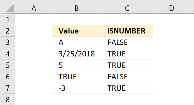
The image above shows the ISNUMBER function in column C. The first value is text value "A" in cell B3, the ISNUMBER function returns FALSE meaning the value is not a number.
The second value in cell B4 contains an Excel date, it contains a number formatted as date. The ISNUMBER function returns TRUE.
The third value is number 5 and the ISNUMBER function returns TRUE, this also applies to negative numbers and 0 (zero).
The fourth value is a boolean value, the ISNUMBER function returns FALSE. Boolean values TRUE and FALSE are not numbers.
Formula in cell D3:
4. Function not working

Check your spelling, a #NAME? error is shown if a function name is unrecognized.

The image above shows the ISNUMBER function returning the boolean value FALSE in cell C4 despite the fact that cell B4 contains a number.

We can see that cell B4 contains an apostrophe before the actual number. This makes Excel identify the number as a text value, however, the apostrophe is not shown in the cell making it very hard to spot.

Excel defaults to right-aligned values for numbers and left-aligned values for text values, see the image above. This is not displayed if you use custom cell formatting.
4.1 Troubleshooting the error value
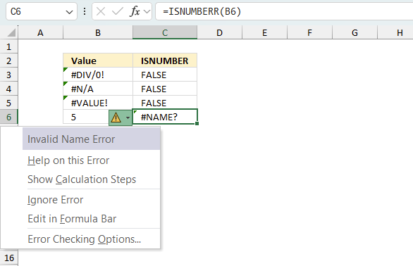
When you encounter an error value in a cell a warning symbol appears, displayed in the image above. Press with mouse on it to see a pop-up menu that lets you get more information about the error.
- The first line describes the error if you press with left mouse button on it.
- The second line opens a pane that explains the error in greater detail.
- The third line takes you to the "Evaluate Formula" tool, a dialog box appears allowing you to examine the formula in greater detail.
- This line lets you ignore the error value meaning the warning icon disappears, however, the error is still in the cell.
- The fifth line lets you edit the formula in the Formula bar.
- The sixth line opens the Excel settings so you can adjust the Error Checking Options.
Here are a few of the most common Excel errors you may encounter.
#NULL error - This error occurs most often if you by mistake use a space character in a formula where it shouldn't be. Excel interprets a space character as an intersection operator. If the ranges don't intersect an #NULL error is returned. The #NULL! error occurs when a formula attempts to calculate the intersection of two ranges that do not actually intersect. This can happen when the wrong range operator is used in the formula, or when the intersection operator (represented by a space character) is used between two ranges that do not overlap. To fix this error double check that the ranges referenced in the formula that use the intersection operator actually have cells in common.
#SPILL error - The #SPILL! error occurs only in version Excel 365 and is caused by a dynamic array being to large, meaning there are cells below and/or to the right that are not empty. This prevents the dynamic array formula expanding into new empty cells.
#DIV/0 error - This error happens if you try to divide a number by 0 (zero) or a value that equates to zero which is not possible mathematically.
#VALUE error - The #VALUE error occurs when a formula has a value that is of the wrong data type. Such as text where a number is expected or when dates are evaluated as text.
#REF error - The #REF error happens when a cell reference is invalid. This can happen if a cell is deleted that is referenced by a formula.
#NAME error - The #NAME error happens if you misspelled a function or a named range.
#NUM error - The #NUM error shows up when you try to use invalid numeric values in formulas, like square root of a negative number.
#N/A error - The #N/A error happens when a value is not available for a formula or found in a given cell range, for example in the VLOOKUP or MATCH functions.
#GETTING_DATA error - The #GETTING_DATA error shows while external sources are loading, this can indicate a delay in fetching the data or that the external source is unavailable right now.
4.2 The formula returns an unexpected value
To understand why a formula returns an unexpected value we need to examine the calculations steps in detail. Luckily, Excel has a tool that is really handy in these situations. Here is how to troubleshoot a formula:
- Select the cell containing the formula you want to examine in detail.
- Go to tab “Formulas” on the ribbon.
- Press with left mouse button on "Evaluate Formula" button. A dialog box appears.
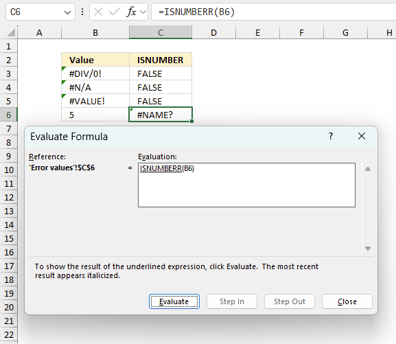
The formula appears in a white field inside the dialog box. Underlined expressions are calculations being processed in the next step. The italicized expression is the most recent result. The buttons at the bottom of the dialog box allows you to evaluate the formula in smaller calculations which you control. - Press with left mouse button on the "Evaluate" button located at the bottom of the dialog box to process the underlined expression.
- Repeat pressing the "Evaluate" button until you have seen all calculations step by step. This allows you to examine the formula in greater detail and hopefully find the culprit.
- Press "Close" button to dismiss the dialog box.
There is also another way to debug formulas using the function key F9. F9 is especially useful if you have a feeling that a specific part of the formula is the issue, this makes it faster than the "Evaluate Formula" tool since you don't need to go through all calculations to find the issue..
- Enter Edit mode: Double-press with left mouse button on the cell or press F2 to enter Edit mode for the formula.
- Select part of the formula: Highlight the specific part of the formula you want to evaluate. You can select and evaluate any part of the formula that could work as a standalone formula.
- Press F9: This will calculate and display the result of just that selected portion.
- Evaluate step-by-step: You can select and evaluate different parts of the formula to see intermediate results.
- Check for errors: This allows you to pinpoint which part of a complex formula may be causing an error.
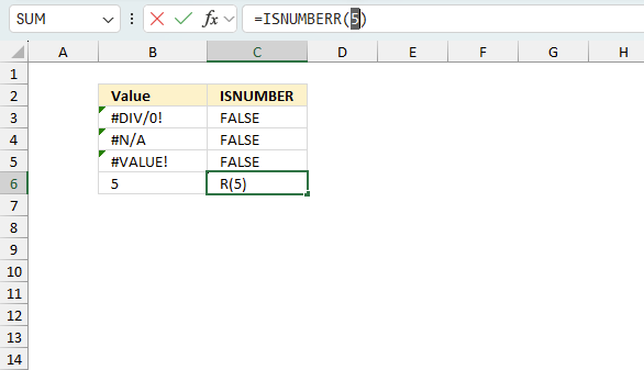
The image above shows cell reference B6 converted to hard-coded value using the F9 key, this value is fine. The ISNUMBER function requires that you spell the function name correctly which is not the case in this example. We have found what is wrong with the formula.
Tips!
- View actual values: Selecting a cell reference and pressing F9 will show the actual values in those cells.
- Exit safely: Press Esc to exit Edit mode without changing the formula. Don't press Enter, as that would replace the formula part with the calculated value.
- Full recalculation: Pressing F9 outside of Edit mode will recalculate all formulas in the workbook.
Remember to be careful not to accidentally overwrite parts of your formula when using F9. Always exit with Esc rather than Enter to preserve the original formula. However, if you make a mistake overwriting the formula it is not the end of the world. You can “undo” the action by pressing keyboard shortcut keys CTRL + z or pressing the “Undo” button
4.3 Other errors
Floating-point arithmetic may give inaccurate results in Excel - Article
Floating-point errors are usually very small, often beyond the 15th decimal place, and in most cases don't affect calculations significantly.
5. Identify numbers stored as text

The image above demonstrates how to identify numbers stored as text in a column, the ISNUMBER function returns FALSE if a value is not a number.
Cell C8 contains boolean value FALSE, the corresponding value in cell B8 contains '-81 which makes Excel think this value is a text value. This may happen if you import data from external sources like databases or web pages.
Formula in cell C3:
It is not necessary to use a formula for each value, you can use a single array formula to process all values in cell range B3:B12. Read the next section to find out how.
5.1 Identify numbers stored as text in a cell range

The array formula in cell D3 checks if the values in cell range B3:B12 are all numbers. It looks like they all are numbers, however, the ISNUMBER function has identified at least one cell value containing a text value.
The formula returns TRUE if all values are numbers and FALSE if at least one value is not a number.
Array formula in cell D3:
5.1.1 How to enter an array formula
Excel 365 users can skip the below steps, enter the formula as a regular formula.

- Doublepress with left mouse button on cell D3 with the left mouse button.
- Enter the above array formula.
- Press and hold CTRL + SHIFT simultaneously.
- Press ENTER once.
- Release all keys.
The array formula begins and ends with curly brackets, see the image above. They appear automatically, don't enter these characters yourself.
5.1.2 Explaining formula in cell D3
Step 1 - Check if the value is a number
ISNUMBER(B3:B12)
becomes
ISNUMBER({-7; 97; 56; 64; -96; "-81"; 62; 99; 57; 85})
and returns
{TRUE; TRUE; TRUE; TRUE; TRUE; FALSE; TRUE; TRUE; TRUE; TRUE}.
Step 2 - Check if all boolean values are TRUE
The AND function returns TRUE if all values are TRUE.
AND(logical1, [logical2], ...)
AND(ISNUMBER(B3:B12))
becomes
AND({TRUE; TRUE; TRUE; TRUE; TRUE; FALSE; TRUE; TRUE; TRUE; TRUE})
and returns FALSE. All values are not TRUE.
6. Highlight numbers stored as text

The image above shows numbers in cell range B3:B12, one cell is highlighted light-grey so you can easily spot non-numbers. Here is how you can do the same:
- Select cell range B3:B12.
- Go to tab "Home" on the ribbon.
- Press with mouse on the "Conditional Formatting" button on the ribbon. A popup menu appears.
- Press with mouse on "New Rule...".

- A dialog box appears. Press with mouse on "Use a formula to determine which cells to format".

- Type the following formula:
=ISNUMBER(B3)=FALSE
- Press with left mouse button on "Format..." button. Another dialog box appears.

- Press with left mouse button on tab "Fill".
- Pick a color to highlight cells with.
- Press with left mouse button on OK button.
- Press with left mouse button on OK button.
6.1 Sort highlighted numbers stored as text

You can sort cells based on cell color to quickly find numbers stored as text in larger data sets. Here is how:
- Select the data range with the mouse.
- Press with right mouse button on on the selected cell range. A popup menu appears.

- Press with mouse on "Sort".
- Press with mouse on "Custom Sort...". A dialog box appears.
- Sort on "Cell Color".
- Pick the color below "Order", see the image below.
- Select "On Top".

- Press with left mouse button on OK.
7. Can the ISNUMBER function handle error values?
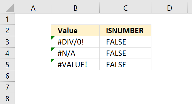
The ISNUMBER function is really useful sometimes because it returns FALSE also from error values, as well. Most Excel functions return an error if they are fed with an error value, however, not all of them.
Most Excel functions that begin with IS handle error values. The image above shows three different error values, #DIV/0, #N/A, and #VALUE! errors. The ISNUMBER function returns FALSE for those values.
8. Identify digits in a string

The image above shows a formula in cell C3 that returns TRUE if at least one character in the string is a digit.
Excel 365 formula in cell C3:
Alternative array formula:
8.1 Explaining formula in cell C3
Step 1 - Count characters
The LEN function returns the number of characters in a given string.
LEN(value)
LEN(B3)
becomes
LEN("Abb")
and returns 3.
Step 2 - Create a sequence of numbers from 1 to n
The SEQUENCE function creates a list of sequential numbers
SEQUENCE(rows, [columns], [start], [step])
SEQUENCE(LEN(B3))
becomes
SEQUENCE(3)
and returns {1; 2; 3}.
Step 3 - Split characters in string one by one
The MID function returns a substring from a string based on the starting position and the number of characters you want to extract.
MID(text, start_num, num_chars)
MID(B3, 1, SEQUENCE(LEN(B3)))
becomes
MID(B3, 1, {1; 2; 3})
becomes
MID("Abb", 1, {1; 2; 3})
and returns {"A"; "b"; "b"}.
Step 4 - Multiply characters by 1
The asterisk character lets you multiply values in an Excel formula. This step is needed in order to convert digits to numbers. For example, "2" becomes 2.
ISNUMBER("2") returns FALSE and we don't want that.
MID(B3, 1, SEQUENCE(LEN(B3)))*1
becomes
{"A"; "b"; "b"}*1
and returns
{#VALUE!; #VALUE!; #VALUE!}. The error value appears when we try to multiply a letter with a number. It is simply not possible.
Step 5 - Check if charcater is a number
ISNUMBER(MID(B3, 1, SEQUENCE(LEN(B3)))*1)
becomes
ISNUMBER({#VALUE!; #VALUE!; #VALUE!})
and returns
{FALSE; FALSE; FALSE}.
Step 6 - Check if at least one character is a digit
The OR function returns TRUE if at least one of the values is TRUE.
OR(ISNUMBER(MID(B3, 1, SEQUENCE(LEN(B3)))*1))
becomes
OR({FALSE; FALSE; FALSE})
and returns FALSE. No digit in this string.
'ISNUMBER' function examples

This post explains how to lookup a value and return multiple values. No array formula required.
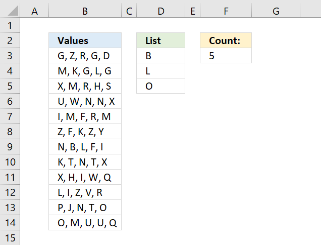
Table of Contents Count cells containing text from list Count entries based on date and time Count cells with text […]
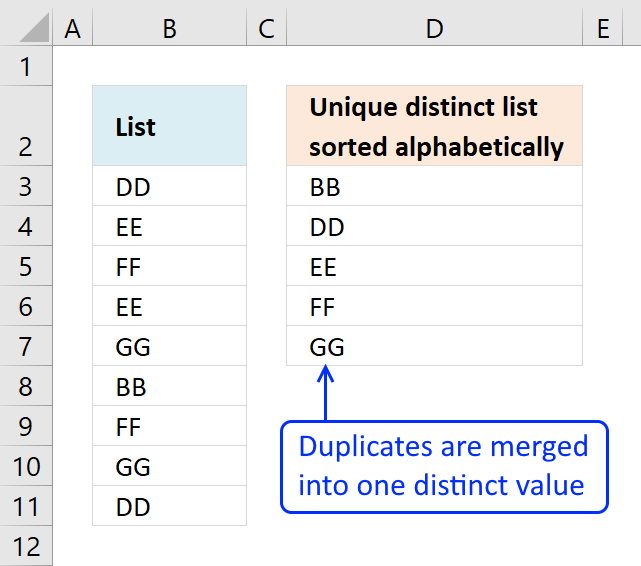
This article demonstrates Excel formulas that allows you to list unique distinct values from a single column and sort them […]
Functions in 'Information' category
The ISNUMBER function function is one of 19 functions in the 'Information' category.
How to comment
How to add a formula to your comment
<code>Insert your formula here.</code>
Convert less than and larger than signs
Use html character entities instead of less than and larger than signs.
< becomes < and > becomes >
How to add VBA code to your comment
[vb 1="vbnet" language=","]
Put your VBA code here.
[/vb]
How to add a picture to your comment:
Upload picture to postimage.org or imgur
Paste image link to your comment.
Contact Oscar
You can contact me through this contact form