How to use the COUNT function
What is the COUNT function?
The COUNT function counts all numerical values in an argument, it allows you to have up to 255 arguments.
Blank cells, boolean values and text values are not counted. It differs from most other functions, ignoring error values.
Table of Contents
- Syntax
- Arguments
- Example
- Count numbers in an array
- Count digits
- Count digits in cell range
- Count negative numbers
- Count positive numbers
- Count numbers in a given range
- Count numbers per row
- Sort rows based on number count
- Count numbers per column
- Sort columns based on number count
- Function not working
- Get Excel *.xlsx file
1. Syntax
COUNT(value1, [value2], ...)
2. Arguments
| value1 | Required. A cell reference, array, or constants for which you want to count numbers. |
| [value2] | Optional. Up to 255 additional arguments. |
3. Example
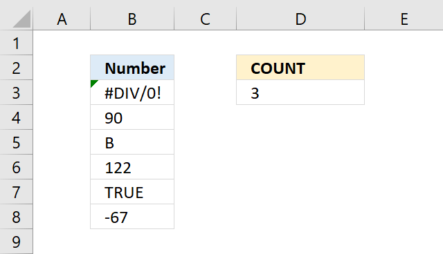
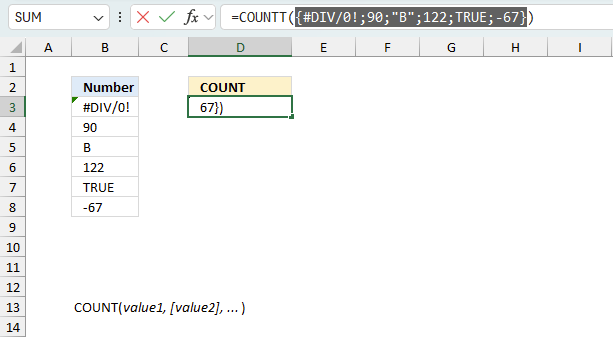
This example demonstrates show the COUNT function works, cell range B3:B8 contains the following values: #DIV/0, 90, B, 122, TRUE, -67
- The first value is a #DIV/0! which is an Excel error. It means that the formula tries to divide number by 0 (zero) which is impossible. The COUNT function ignores error values.
- The second value is 90 which is a number. This is the first number.
- The third value is "B" which is a text value, this value is not added to the total count because it is not a numerical value.
- The fourth value is 122 which is a number. This is the second number in the list.
- The fifth value is TRUE which is a boolean value meaning it is not a numerical value. This value is also ignored.
- The sixth value is -67 which is a numerical value and is added to the total.
Formula in cell D3:
The formula in cell D3 returns 3 meaning the list in cell B3:B8 contains 3 numerical value or numbers. Use the COUNT function to count numbers in a cell range, this is great for verifying that you got the correct number of numerical values in the specified cell range.
3.1 Explaining formula
COUNT(B3:B8)
becomes
COUNT({#DIV/0!;90;"B";122;TRUE;-67})
and returns 3. There are three numbers in cell range B3:B8, they are 90, 122, and -67.
4. Count numbers in an array

The COUNT function works fine with constants in an array as well, in other words, the COUNT function counts numerical values or numbers in hard-coded values or constants in a formula.
The formula below shows how to hard-code values, text values must have a beginning and ending double quote or the formula will returns a #NAME! error. This means that the Excel thinks you have entered a misspelled function.
Multiple hard-coded values must be entered with beginning and ending curly brackets. The tell Excel that this is an array of values, use specific characters to delimit values by row or column. These specific charcaters are determined by your regional settings. For example, US has a comma as a column delimiter and a semicolon as a delimiter for rows.
Formula in cell B3:
The array in the formula above has three values, two numerical values and one text value. There are two numbers in {1,"A",-5}, they are 1 and -5. The formula returns 2 which represents two numerical values.
5. Count digits in a cell

The following example demonstrates how to count digits in a cell value. Cell B3 contains "A45BV23XC2", the formula in cell D3 splits the string into one character each returning an array containing single characters in each container.
The COUNT function counts the numerical values in the array and returns the total number of numbers. I have bolded the numerical digits in the array: {"A";"4";"5";"B";"V";"2";"3";"X";"C";"2"}
Formula in cell D3:
The numbers in the array are 4, 5, 2, 3, and 2. The total number in the array is 5 which is what the formula returns in cell D3.
5.1 Explaining formula
Step 1 - Count characters in cell
The LEN function returns the number of characters in a cell value.
LEN(text)
LEN(B3)
becomes
LEN("A45BV23XC2")
and returns 10. There are ten characters in cell B3.
Step 2 - Create numbers from 1 to n
The SEQUENCE function creates a list of sequential numbers.
SEQUENCE(rows, [columns], [start], [step])
SEQUENCE(LEN(B3))
becomes
SEQUENCE(10)
and returns
{1; 2; 3; 4; 5; 6; 7; 8; 9; 10}.
Step 3 - Split characters into an array
The MID function returns a substring from a string based on the starting position and the number of characters you want to extract.
MID(text, start_num, num_chars)
MID(B3,SEQUENCE(LEN(B3)),1)
becomes
MID(B3,{1; 2; 3; 4; 5; 6; 7; 8; 9; 10},1)
becomes
MID("A45BV23XC2",{1; 2; 3; 4; 5; 6; 7; 8; 9; 10},1)
and returns
{"A"; "4"; "5"; "B"; "V"; "2"; "3"; "X"; "C"; "2"}.
Step 4 - Convert text numbers to numbers
The asterisk lets you multiply numbers in an Excel formula, it also lets you convert "text" numbers to regular numbers.
MID(B3,SEQUENCE(LEN(B3)),1)*1
becomes
{"A"; "4"; "5"; "B"; "V"; "2"; "3"; "X"; "C"; "2"}*1
and returns
{#VALUE!; 4; 5; #VALUE!; #VALUE!; 2; 3; #VALUE!; #VALUE!; 2}.
Note the numbers are not enclosed by double quotes any more. The text values are now error values but that changes nothing, the COUNT function ignores error values.
Step 5 - Count numbers in array
COUNT(MID(B3,SEQUENCE(LEN(B3)),1)*1)
becomes
COUNT({#VALUE!; 4; 5; #VALUE!; #VALUE!; 2; 3; #VALUE!; #VALUE!; 2})
and returns 5.

6. Count digits in a cell range

This example counts all numerical values in a given cell range, the formula in section 5 counts only numerical values in one given cell. The TEXTJOIN function joins all strings in cell range B3:B13.
The formula then splits the joined text string into an array containing a single character in each container. The COUNT function counts all containers containing a numerical value, in other words, a number.
Formula in cell D3:
The following subsection 6.1 explains in greater detail how the formula works.
6.1 Explaining formula
Step 1 - Join values in cell range B3:B13
The TEXTJOIN function combines text strings from multiple cell ranges and also delimiting characters.
TEXTJOIN(delimiter, ignore_empty, text1, [text2], ...)
TEXTJOIN(, TRUE, B3:B13)
becomes
TEXTJOIN(, TRUE, {"KHFV9Z89Y"; "8VUKTKECVP"; ... ; "294RZ652J8S4UHT"})
and returns
"KHFV...UHT".
Step 2 - Count characters in string
The LEN function returns the number of characters in a cell value.
LEN(text)
LEN(TEXTJOIN(, TRUE, B3:B13))
becomes
LEN("KHFV...UHT")
and returns 116. There is a total of 116 characters in the string.
Step 3 - Create numbers from 1 to n
The SEQUENCE function creates a list of sequential numbers.
SEQUENCE(rows, [columns], [start], [step])
SEQUENCE(LEN(TEXTJOIN(, TRUE, B3:B13)))
becomes
SEQUENCE(116)
and returns {1;2;3;...;116}.
Step 4 - Split string
The MID function returns a substring from a string based on the starting position and the number of characters you want to extract.
MID(text, start_num, num_chars)
MID(TEXTJOIN(, TRUE, B3:B13), SEQUENCE(LEN(TEXTJOIN(, TRUE, B3:B13))), 1)
becomes
MID("KHFV...UHT", {1;2;3;...;116}, 1)
and returns
{"K";"H";"F";...;"T"}
Step 5 - Convert text numbers to regular numbers
The asterisk lets you multiply numbers in an Excel formula, it also lets you convert "text" numbers to regular numbers.
MID(TEXTJOIN(, TRUE, B3:B13), SEQUENCE(LEN(TEXTJOIN(, TRUE, B3:B13))), 1)*1
becomes
{"K";"H";"F";...;"T"}*1
and returns
{#VALUE!;#VALUE!;#VALUE!;...;#VALUE!}
Step 6 - Count numbers
COUNT(MID(TEXTJOIN(, TRUE, B3:B13), SEQUENCE(LEN(TEXTJOIN(, TRUE, B3:B13))), 1)*1)
becomes
COUNT({#VALUE!;#VALUE!;#VALUE!;...;#VALUE!})
and returns 41. There are 41 digits in cell range B3:B13.
7. Count negative numbers

The COUNT function can count negative numbers in a given cell range, however, you need some additional functions or clever workarounds.
Formula in cell D3:
I recommend using the COUNTIF function, it is built to count values in a cell range based on a given condition. The formula stays small and easy to understand, just the way we like it.
The COUNTIF function lets you specify a condition in the second argument. which in this case is "<0". The < character is a comparison character that checks if the cell values in cell range B3:B8 is smaller than 0 (zero), in other words, negative values.
Cell range B3:B8 contains the following values: #DIV/0, 90, B, 122, TRUE, -67. Only one value is a negative number: -67. The formula in cell D3 returns 1 representing the number of negative values in cell range B3:B8.
7.1 Explaining formula
The COUNTIF function calculates the number of cells that meet a condition.
COUNTIF(range, criteria)
COUNTIF(B3:B8, "<0")
becomes
COUNTIF({#DIV/0!;90;"B";122;TRUE;-67}, "<0")
and returns 1. -67 is the only negative number in the array.
8. Count positive numbers

The image above demonstrates a formula that counts positive numerical values. Cell range B3:B8 contains the following values: #DIV/0, 90, B, 122, TRUE, -67
Only values 90 and 122 are positive numbers, the remaining are negative values, boolean value, and an error value.
Formula in cell D3:
The COUNTIF function lets you specify a condition in the second argument. which in this case is ">0". The > character is a comparison character that checks if the cell values in cell range B3:B8 are larger than 0 (zero), in other words, positive numbers.
The formula in cell D3 returns 2 representing the total number of positive numbers in cell range B3:B8.
8.1 Explaining formula
The COUNTIF function calculates the number of cells that meet a condition.
COUNTIF(range, criteria)
COUNTIF(B3:B8, ">0")
becomes
COUNTIF({#DIV/0!;90;"B";122;TRUE;-67}, ">0")
and returns 2. 90 and 122 are larger than 0 (zero).
9. Count numbers in a given range

This examples show how to count numbers between a given numerical range in a specific cell range. The COUNT function can do this as well, however, there is a function built for two or more conditions. Cell range B3:B8 contains the following values: #DIV/0, 90, B, 122, TRUE, -67.
Formula in cell D3:
The formula above uses two conditions to count the numerical values in B3:B8, they are: ">80" meaning values larger than 80 and "<150" meaning numbers smaller than 150. Both conditions must be met in order for a value to be included into the count.
The formula in cell D3 returns 2 representing the total number of values smaller than 150 and larger than 80, in cell range B3:B8.
9.1 Explaining formula
The COUNTIFS function calculates the number of cells across multiple ranges that equals all given conditions.
COUNTIFS(criteria_range1, criteria1, [criteria_range2, criteria2]…)
COUNTIFS(B3:B8, ">80",B3:B8, "<150")
becomes
COUNTIFS({#DIV/0!;90;"B";122;TRUE;-67}, ">80",{#DIV/0!;90;"B";122;TRUE;-67}, "<150")
and returns 2. 90 and 122 are larger than 80 and smaller than 150.
10. Count numbers per row

The image above shows an Excel 365 dynamic array formula that calculates how many numbers there are on each row in cell range B3:E9. In other words, the formula returns an array of values in cell G3 and spills values to cells below as far as needed.
The array has values that match the rows in B3:E9, each number represents the number of numerical values for that particular row.
Excel 365 formula in cell G3:
For example, row 3 has the following values: "VATE", "RVEO", 86, and 20. Only two values are numbers so the formula returns two in cell G3.
What is special about the BYROW function is that it performs the calculation for the entire range B3:E9 which is harder but doable in earlier Excel versions using the MMULT function etc.
Explaining formula
Step 1 - Count cells only numbers
The COUNT function counts all numerical values in an argument.
Function syntax: COUNT(value1, [value2], ...)
COUNT(a)
Step 2 - Build the LAMBDA function
The LAMBDA function build custom functions without VBA, macros or javascript.
Function syntax: LAMBDA([parameter1, parameter2, …,] calculation)
LAMBDA(a,COUNT(a))
Step 3 - Count nonempty cells per row
The BYROW function puts values from an array into a LAMBDA function row-wise.
Function syntax: BYROW(array, lambda(array, calculation))
BYROW(B3:E9,LAMBDA(a,COUNT(a)))
11. Sort rows based on number count

This example builds on the example above in section 10, we discussed how to count the number of numerical values per row and demonstrated a formula.
This formula below sorts the rows in B3:E9 based on the count of numerical values. For example, row 7 in B3:E9 contains three separate numbers making it the row with the highest count.
Excel 365 dynamic array formula in cell G3:
The formula in cell G3 returns row 7 at the top and then continues with rows with a lower count. The last three rows has only one number and they are rows 6, 8, and 9 in B3:E9.
Also, the Excel 365 formula spills values below and to the right as far as needed. A #SPILL! error is shown if those destinations cells are not empty. Column K shows the count next to the sorted output.
Explaining formula
This formula works just like the example in section 10, but it also sorts rows based on the count of cells containing only numbers. The values in G3:J3 has three numbers, 87, 86, and 67. That row has the largest number of numerical values in B3:E9 shown in cell K3.
The SORTBY function sorts a cell range or array based on values in a corresponding range or array.
Function syntax: SORTBY(array, by_array1, [sort_order1], [by_array2, sort_order2],…)
12. Count numbers per column

The image above shows an Excel 365 dynamic array formula in cell B11 that counts numbers per column in cell range B3:E9. This is similar to to the formula in section 10, however, this calculates the number of numerical values per column instead of per row.
The formula returns an array that has the same number of columns as the source data range B3:E9. This means that the formula spills values to the right as far as needed.
Excel 365 formula in cell B11:
The first column two numerical values, cell B4: 47 and cell B7: 87. The next column has only one numerical value, the remaining values are text strings, 40 is found in cell C5.
The third column contains 5 numerical values, cell D3: 86, cell D4: 60, cell D6: 14, cell D7: 86, and D8: 13. The last column has 4 numerical values in cells E3, E5, E7, and E9. They are respectively 20, 5, 67, and 64.
Explaining formula
Step 1 - Count numbers
The COUNT function counts all numerical values in an argument.
Function syntax: COUNT(value1, [value2], ...)
COUNT(a)
Step 2 - Build the LAMBDA function
The LAMBDA function build custom functions without VBA, macros or javascript.
Function syntax: LAMBDA([parameter1, parameter2, …,] calculation)
LAMBDA(a,COUNT(a))
Step 3 - Count numbers per column
The BYCOL function passes all values in a column based on an array to a LAMBDA function, the LAMBDA function calculates new values based on a formula you specify.
Function syntax: BYCOL(array, lambda(array, calculation))
BYCOL(B3:E9,LAMBDA(a,COUNT(a)))
13. Sort columns based on number count

Excel 365 dynamic array formula in cell G3:
Explaining formula
This formula works just like the example in section 12, however, it also sorts the columns based on the number of cells containing only numbers.
The image above shows 5 in cell G11, and there are five numbers cells in G3:G9. The next cell H11 displays 4, there are four cells in H3:H9 containing only numbers.
The SORTBY function sorts a cell range or array based on values in a corresponding range or array.
Function syntax: SORTBY(array, by_array1, [sort_order1], [by_array2, sort_order2],…)
14. Function not working
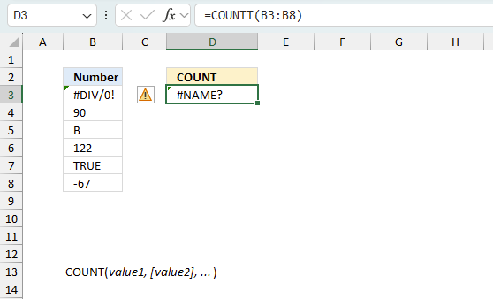
The COUNT function returns #NAME? error if you misspell the function name. It doesn't propagate errors, meaning that if the input contains an error (e.g., #VALUE!, #REF!) the function will return the same error.
14.1 Troubleshooting the error value
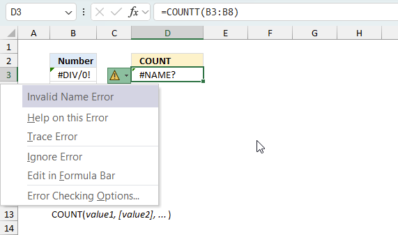
When you encounter an error value in a cell a warning symbol appears, displayed in the image above. Press with mouse on it to see a pop-up menu that lets you get more information about the error.
- The first line describes the error if you press with left mouse button on it.
- The second line opens a pane that explains the error in greater detail.
- The third line takes you to the "Evaluate Formula" tool, a dialog box appears allowing you to examine the formula in greater detail.
- This line lets you ignore the error value meaning the warning icon disappears, however, the error is still in the cell.
- The fifth line lets you edit the formula in the Formula bar.
- The sixth line opens the Excel settings so you can adjust the Error Checking Options.
Here are a few of the most common Excel errors you may encounter.
#NULL error - This error occurs most often if you by mistake use a space character in a formula where it shouldn't be. Excel interprets a space character as an intersection operator. If the ranges don't intersect an #NULL error is returned. The #NULL! error occurs when a formula attempts to calculate the intersection of two ranges that do not actually intersect. This can happen when the wrong range operator is used in the formula, or when the intersection operator (represented by a space character) is used between two ranges that do not overlap. To fix this error double check that the ranges referenced in the formula that use the intersection operator actually have cells in common.
#SPILL error - The #SPILL! error occurs only in version Excel 365 and is caused by a dynamic array being to large, meaning there are cells below and/or to the right that are not empty. This prevents the dynamic array formula expanding into new empty cells.
#DIV/0 error - This error happens if you try to divide a number by 0 (zero) or a value that equates to zero which is not possible mathematically.
#VALUE error - The #VALUE error occurs when a formula has a value that is of the wrong data type. Such as text where a number is expected or when dates are evaluated as text.
#REF error - The #REF error happens when a cell reference is invalid. This can happen if a cell is deleted that is referenced by a formula.
#NAME error - The #NAME error happens if you misspelled a function or a named range.
#NUM error - The #NUM error shows up when you try to use invalid numeric values in formulas, like square root of a negative number.
#N/A error - The #N/A error happens when a value is not available for a formula or found in a given cell range, for example in the VLOOKUP or MATCH functions.
#GETTING_DATA error - The #GETTING_DATA error shows while external sources are loading, this can indicate a delay in fetching the data or that the external source is unavailable right now.
14.2 The formula returns an unexpected value
To understand why a formula returns an unexpected value we need to examine the calculations steps in detail. Luckily, Excel has a tool that is really handy in these situations. Here is how to troubleshoot a formula:
- Select the cell containing the formula you want to examine in detail.
- Go to tab “Formulas” on the ribbon.
- Press with left mouse button on "Evaluate Formula" button. A dialog box appears.
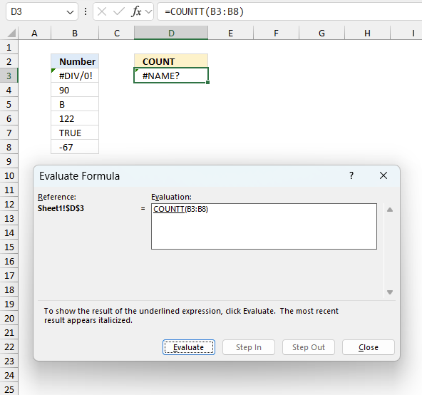
The formula appears in a white field inside the dialog box. Underlined expressions are calculations being processed in the next step. The italicized expression is the most recent result. The buttons at the bottom of the dialog box allows you to evaluate the formula in smaller calculations which you control. - Press with left mouse button on the "Evaluate" button located at the bottom of the dialog box to process the underlined expression.
- Repeat pressing the "Evaluate" button until you have seen all calculations step by step. This allows you to examine the formula in greater detail and hopefully find the culprit.
- Press "Close" button to dismiss the dialog box.
There is also another way to debug formulas using the function key F9. F9 is especially useful if you have a feeling that a specific part of the formula is the issue, this makes it faster than the "Evaluate Formula" tool since you don't need to go through all calculations to find the issue..
- Enter Edit mode: Double-press with left mouse button on the cell or press F2 to enter Edit mode for the formula.
- Select part of the formula: Highlight the specific part of the formula you want to evaluate. You can select and evaluate any part of the formula that could work as a standalone formula.
- Press F9: This will calculate and display the result of just that selected portion.
- Evaluate step-by-step: You can select and evaluate different parts of the formula to see intermediate results.
- Check for errors: This allows you to pinpoint which part of a complex formula may be causing an error.
The image above shows cell reference B3:B8 converted to hard-coded value using the F9 key, however, there is nothing wrong with these values. The COUNT function requires you to spell the name correctly which is not the case in this example. We have found what is wrong with the formula.
Tips!
- View actual values: Selecting a cell reference and pressing F9 will show the actual values in those cells.
- Exit safely: Press Esc to exit Edit mode without changing the formula. Don't press Enter, as that would replace the formula part with the calculated value.
- Full recalculation: Pressing F9 outside of Edit mode will recalculate all formulas in the workbook.
Remember to be careful not to accidentally overwrite parts of your formula when using F9. Always exit with Esc rather than Enter to preserve the original formula. However, if you make a mistake overwriting the formula it is not the end of the world. You can “undo” the action by pressing keyboard shortcut keys CTRL + z or pressing the “Undo” button
14.3 Other errors
Floating-point arithmetic may give inaccurate results in Excel - Article
Floating-point errors are usually very small, often beyond the 15th decimal place, and in most cases don't affect calculations significantly.
'COUNT' function examples
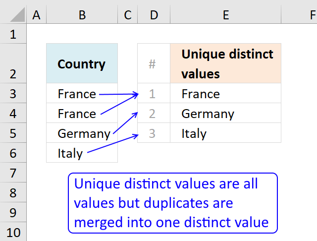
This article describes how to count unique distinct values. What are unique distinct values? They are all values but duplicates are […]
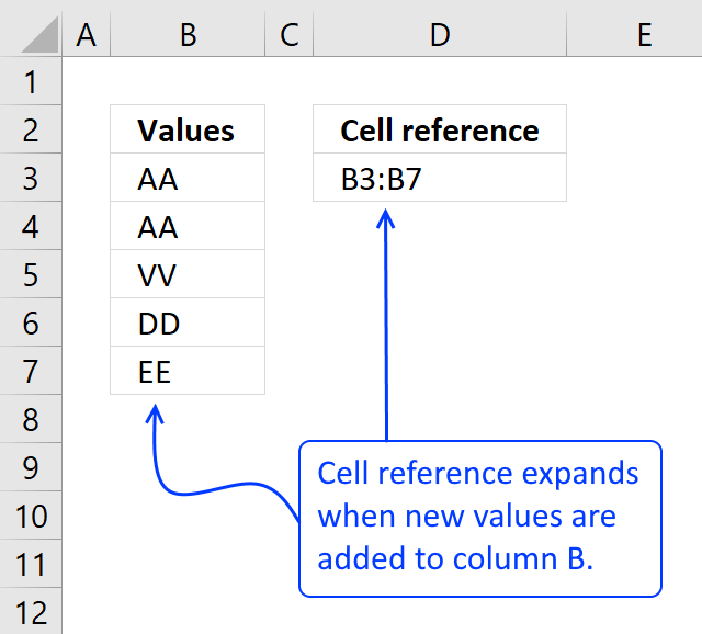
What is a named range? A named range is a feature in Excel that allows you to assign a specific […]
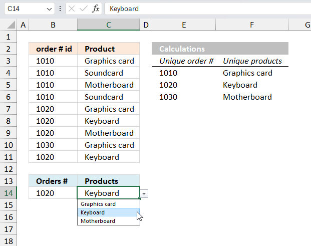
Table of Contents Create dependent drop down lists containing unique distinct values - Excel 365 Create dependent drop down lists […]
Functions in 'Statistical' category
The COUNT function function is one of 73 functions in the 'Statistical' category.
How to comment
How to add a formula to your comment
<code>Insert your formula here.</code>
Convert less than and larger than signs
Use html character entities instead of less than and larger than signs.
< becomes < and > becomes >
How to add VBA code to your comment
[vb 1="vbnet" language=","]
Put your VBA code here.
[/vb]
How to add a picture to your comment:
Upload picture to postimage.org or imgur
Paste image link to your comment.
Contact Oscar
You can contact me through this contact form