How to use the SEARCH function

What is the SEARCH function?
The SEARCH function returns a number representing the position of character at which a specific text string is found reading left to right. It is not a case-sensitive search.
Table of Contents
1. Syntax
SEARCH(find_text,within_text, [start_num])
2. Arguments
| find_text | Required. Is the text you want to find. Wildcard characters (? and *) are allowed. |
| within_text | Required. Is the text in which you want to search for find_text. |
| [start_num] | Optional. Is the character number in within_text, counting from the left at which you want to start searching. If omitted 1 is used. |
3. Example
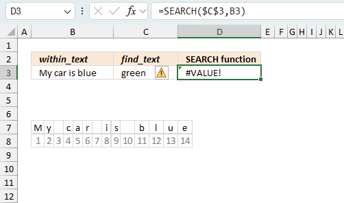
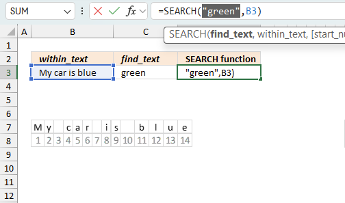
The image above demonstrates the function in cell D3.
The first argument find_text is a cell reference to the value in cell C3, the function will look for the value specified in cell C3 in the value in cell B3.
It returns number 11 in this example. Text string "blue" is found in position 11 if you count characters from left to right "My car is blue".
Row 7 shows the text string with a single character in each cell, row 8 shows the count for each cell.

The SEARCH function is not case sensitive, use the FIND function if lower and upper case letters are important.
The image above shows that using a text string in uppercase letters (cell C3) still matches the text in cell B3.
Formula in cell C3:
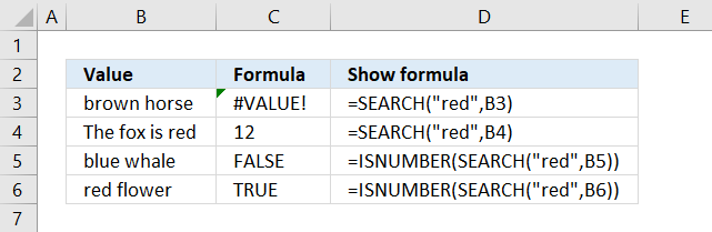
If the text string is not found the SEARCH function returns a #VALUE! error. The image above shows the erro output from the SEARCH function in cell C3.
Text string "red" is not found in cell B3 "brown horse", the issue with error values is that they break a formula, however, there are workarounds.
Use the ISNUMBER function to avoid breaking the formula. It returns TRUE if the returned value is a number and FALSE for everything else even errors.
Formula in cell C5:
ISNUMBER(SEARCH("red", B5))
becomes
ISNUMBER(SEARCH("red", "blue whale"))
becomes
ISNUMBER(#VALUE!)
and returns FALSE in cell C5.
4. Function not working
The SEARCH function returns a
- #VALUE! error if the string is not found.
- #NAME? error if you misspell the function name.
- propagates errors, meaning that if the input contains an error (e.g., #VALUE!, #REF!), the function will return the same error.
4.1 Troubleshooting the error value
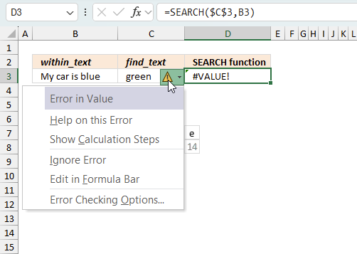
When you encounter an error value in a cell a warning symbol appears, displayed in the image above. Press with mouse on it to see a pop-up menu that lets you get more information about the error.
- The first line describes the error if you press with left mouse button on it.
- The second line opens a pane that explains the error in greater detail.
- The third line takes you to the "Evaluate Formula" tool, a dialog box appears allowing you to examine the formula in greater detail.
- This line lets you ignore the error value meaning the warning icon disappears, however, the error is still in the cell.
- The fifth line lets you edit the formula in the Formula bar.
- The sixth line opens the Excel settings so you can adjust the Error Checking Options.
Here are a few of the most common Excel errors you may encounter.
#NULL error - This error occurs most often if you by mistake use a space character in a formula where it shouldn't be. Excel interprets a space character as an intersection operator. If the ranges don't intersect an #NULL error is returned. The #NULL! error occurs when a formula attempts to calculate the intersection of two ranges that do not actually intersect. This can happen when the wrong range operator is used in the formula, or when the intersection operator (represented by a space character) is used between two ranges that do not overlap. To fix this error double check that the ranges referenced in the formula that use the intersection operator actually have cells in common.
#SPILL error - The #SPILL! error occurs only in version Excel 365 and is caused by a dynamic array being to large, meaning there are cells below and/or to the right that are not empty. This prevents the dynamic array formula expanding into new empty cells.
#DIV/0 error - This error happens if you try to divide a number by 0 (zero) or a value that equates to zero which is not possible mathematically.
#VALUE error - The #VALUE error occurs when a formula has a value that is of the wrong data type. Such as text where a number is expected or when dates are evaluated as text.
#REF error - The #REF error happens when a cell reference is invalid. This can happen if a cell is deleted that is referenced by a formula.
#NAME error - The #NAME error happens if you misspelled a function or a named range.
#NUM error - The #NUM error shows up when you try to use invalid numeric values in formulas, like square root of a negative number.
#N/A error - The #N/A error happens when a value is not available for a formula or found in a given cell range, for example in the VLOOKUP or MATCH functions.
#GETTING_DATA error - The #GETTING_DATA error shows while external sources are loading, this can indicate a delay in fetching the data or that the external source is unavailable right now.
4.2 The formula returns an unexpected value
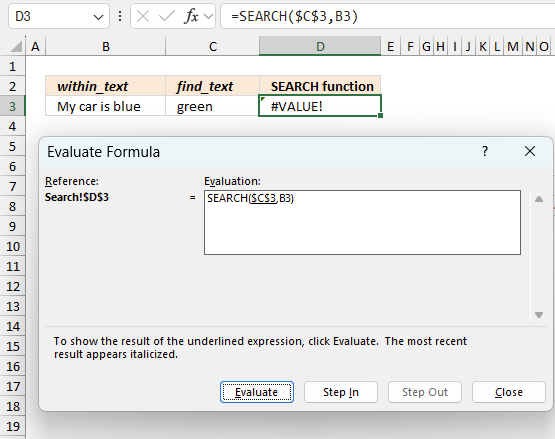
To understand why a formula returns an unexpected value we need to examine the calculations steps in detail. Luckily, Excel has a tool that is really handy in these situations. Here is how to troubleshoot a formula:
- Select the cell containing the formula you want to examine in detail.
- Go to tab “Formulas” on the ribbon.
- Press with left mouse button on "Evaluate Formula" button. A dialog box appears.
The formula appears in a white field inside the dialog box. Underlined expressions are calculations being processed in the next step. The italicized expression is the most recent result. The buttons at the bottom of the dialog box allows you to evaluate the formula in smaller calculations which you control. - Press with left mouse button on the "Evaluate" button located at the bottom of the dialog box to process the underlined expression.
- Repeat pressing the "Evaluate" button until you have seen all calculations step by step. This allows you to examine the formula in greater detail and hopefully find the culprit.
- Press "Close" button to dismiss the dialog box.
There is also another way to debug formulas using the function key F9. F9 is especially useful if you have a feeling that a specific part of the formula is the issue, this makes it faster than the "Evaluate Formula" tool since you don't need to go through all calculations to find the issue..
- Enter Edit mode: Double-press with left mouse button on the cell or press F2 to enter Edit mode for the formula.
- Select part of the formula: Highlight the specific part of the formula you want to evaluate. You can select and evaluate any part of the formula that could work as a standalone formula.
- Press F9: This will calculate and display the result of just that selected portion.
- Evaluate step-by-step: You can select and evaluate different parts of the formula to see intermediate results.
- Check for errors: This allows you to pinpoint which part of a complex formula may be causing an error.
The image above shows cell reference C3 converted to hard-coded value using the F9 key. The SEARCH function requires a valid find_text argument value which is not the case in this example. We have found what is wrong with the formula.
Tips!
- View actual values: Selecting a cell reference and pressing F9 will show the actual values in those cells.
- Exit safely: Press Esc to exit Edit mode without changing the formula. Don't press Enter, as that would replace the formula part with the calculated value.
- Full recalculation: Pressing F9 outside of Edit mode will recalculate all formulas in the workbook.
Remember to be careful not to accidentally overwrite parts of your formula when using F9. Always exit with Esc rather than Enter to preserve the original formula. However, if you make a mistake overwriting the formula it is not the end of the world. You can “undo” the action by pressing keyboard shortcut keys CTRL + z or pressing the “Undo” button
4.3 Other errors
Floating-point arithmetic may give inaccurate results in Excel - Article
Floating-point errors are usually very small, often beyond the 15th decimal place, and in most cases don't affect calculations significantly.
5. Wildcard characters

There are two wildcard characters you can use in the SEARCH function.
| Character | Wildcard | Description |
| * | asterisk | Matches 0 (zero) to any number of characters. |
| ? | question mark | Matches one character only. |
Formula in cell D3:
The SEARCH function in cell D3 returns 1, cell C3 contains *blue. The asterisk matches any number of characters even 0 (zero).
*blue matches the entire text string in cell B3 "My car is blue" and therefore matches the first character and returns 1.
Formula in cell D4:
Cell C4 contains blue* and matches at the eleventh character, the asterisk matches any number of characters from zero and up.
Formula in cell D5:
The question mark character matches any single character, ?blue matches "My car is blue" at the tenth character. The ? matches the blank (space) as well and the SEARCH function returns 10.
Formula in cell D6:
blue? doesn't match text "My car is blue" and returns #VALUE! error. The question mark matches any single character but string "My car is blue" has no character after blue.
6. Count how many times a specific string is found in a cell using the SEARCH function?

You can't use the SEARCH function to count how many time a specific string exists in a cell, it will only return the number of the character of the string that first matches, reading from left to right.
This article explains how to Count specific text string in a cell.
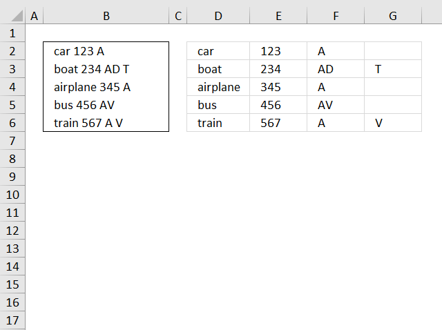
7. Can you count how many times a specific string is found in a cell range using the SEARCH function?

Yes, but only one instance per cell. Formula in cell D3:
If you are an Excel 365 subscriber you can use the regular formula above. Excel users with previous versions can use the formula below.
Let me explain how these two formula work.
SEARCH(C3,B3:B5)
becomes
SEARCH("aa", {"aa bb cc aa dd"; "bb cc dd"; "aa bb cc aa dd"})
and returns {1; #VALUE!; 1}. The numbers indicate that a matching string is found.
ISNUMBER(SEARCH(C3,B3:B5))
becomes
ISNUMBER({1; #VALUE!; 1})
and returns {TRUE; FALSE; TRUE}. The SUM and SUMPRODUCT functions can't sum add boolean values, to convert boolean values to numbers simply multiply with 1.
ISNUMBER(SEARCH(C3,B3:B5))*1
becomes
{TRUE; FALSE; TRUE}*1
and returns {1;0;1}. 1 is the equivalent of boolean value TRUE and 0 (zero) is boolean value FALSE.
8. SEARCH function with multiple search values?

You can use multiple text strings, however, if there are more than one instance of a specific string only one is counted.
For example cell B3 contains two "aa" but the formula in cell D3 counts only one instance.
The formula returns 2 because text strings "aa" and "bb" are found in cell B3. The formula is exactly the same as the one above so I won't explain it again, however, note that the cell references are different.
9. How to get the position of the second instance?

The string "aa" we are looking for exists twice in cell B3, the following formula returns a number representing the position of the character of the string the second time it occurs.
This formula changes the first instance to another string so that the SEARCH function then finds the position of the second instance of the string we are looking for.
SEARCH(C3,B3) finds the position of the first instance, it returns 1. The REPLACE function then changes the first string to something else, in this case, character "|". If your cell contains this character already then I recommend changing it to something that is not used in the cell so the formula doesn't get confused.
REPLACE(B3,SEARCH(C3,B3),LEN(C3),REPT("|", LEN(C3)))
becomes
REPLACE(B3,SEARCH(C3,B3),LEN(C3),REPT("|", LEN("aa")))
becomes
REPLACE(B3,SEARCH(C3,B3),LEN(C3),REPT("|", 2))
becomes
REPLACE(B3,SEARCH(C3,B3),LEN(C3),"||")
becomes
REPLACE(B3,SEARCH(C3,B3),2,"||")
becomes
REPLACE(B3,1,2,"||")
becomes
REPLACE("aa bb cc aa dd",1,2,"||")
and returns "|| bb cc aa dd".
SEARCH(C3,REPLACE(B3,SEARCH(C3,B3),LEN(C3),REPT("|", LEN(C3))))
becomes
SEARCH(C3,"|| bb cc aa dd")
and returns 10 in cell D3.
10. How to get the relative position of all instances?

The following formula works only in Excel 365, it returns numbers representing the position of the found instances in a cell.
Dynamic array formula in cell C3:
7.1 Explaining formula in cell C3
Step 1 - Calculate the number of characters in a given cell
LEN(B3)
Step 2 - Create a sequence from 1 to n
SEQUENCE(LEN(B3))
Step 3 - Create an array of substrings
MID(B3, SEQUENCE(LEN(B3)), LEN(E3))
Step 4 - Compare substrings to condition
MID(B3, SEQUENCE(LEN(B3)), LEN(E3))=E3
Step 5 - Filter corresponding numbers
FILTER(SEQUENCE(LEN(B3)), MID(B3, SEQUENCE(LEN(B3)), LEN(E3))=E3)
Step 6 - Concatenate strings
TEXTJOIN(", ", TRUE, FILTER(SEQUENCE(LEN(B3)), MID(B3, SEQUENCE(LEN(B3)), LEN(E3))=E3))
'SEARCH' function examples

This post explains how to lookup a value and return multiple values. No array formula required.
This blog article describes how to split strings in a cell with space as a delimiting character, like Text to […]
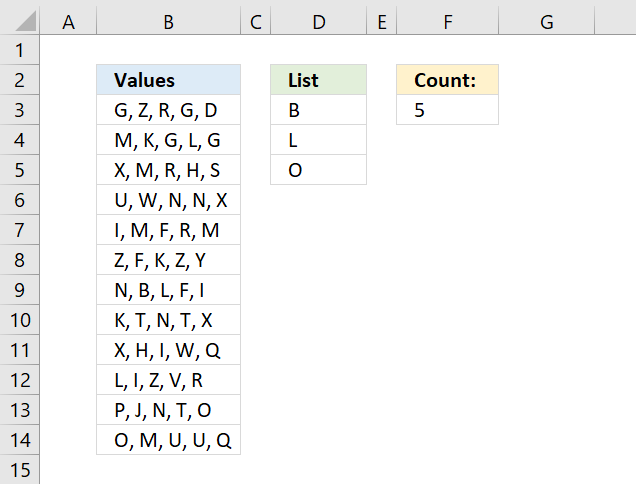
Table of Contents Count cells containing text from list Count entries based on date and time Count cells with text […]
Functions in 'Text' category
The SEARCH function function is one of 29 functions in the 'Text' category.
Excel function categories
Excel categories
3 Responses to “How to use the SEARCH function”
Leave a Reply
How to comment
How to add a formula to your comment
<code>Insert your formula here.</code>
Convert less than and larger than signs
Use html character entities instead of less than and larger than signs.
< becomes < and > becomes >
How to add VBA code to your comment
[vb 1="vbnet" language=","]
Put your VBA code here.
[/vb]
How to add a picture to your comment:
Upload picture to postimage.org or imgur
Paste image link to your comment.
Just an additon..
"The function works the same as the search function except case-sensitive" & Find doesn't works with wildcard characters — the question mark (?) and asterisk (*) where SEARCH can.. :)
Regards,
Deb
Thank you, Deb!
[…] SEARCH(find_text,within_text, [start_num]) Returns the number of the character at which a specific character or text string is first found, reading left to right (not case sensitive) […]