Rearrange values using formulas
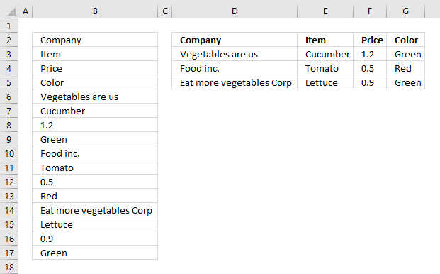
The picture above shows data presented in only one column (column B), this happens sometimes when you get an undesired output from a database or copying values from an HTML file.
The formula in cell D2 extracts values from column B to a cell range containing four columns and 4 rows.
What's on this page
1. Rearrange values from a single column cell range to many columns
The INDEX function allows you to easily rearrange values on an Excel worksheet, in this case, data seems to be grouped record by record. 4 values in one record. Column D to G shows you the INDEX function rearranging the data.
The INDEX function has three arguments: INDEX(reference, row_num, [column_num])
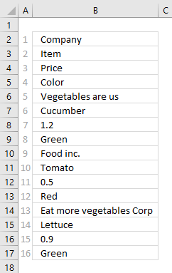
The reference in the first argument points to cell range B2:B17. To return a value from that cell range you must know where it is, the INDEX function uses a row and column number to locate a particular value. Since this cell range (B2:B17) only has one column you only need to use a row number to get the value you want.
The picture above has relative row numbers in column A to show you what number the INDEX function needs for it to return a specific value from cell range B2:B17. The values in column B seems to repeat, every 4th row has a company name. We can use that information to build the formula that returns a record in a row each.
The formula needs numbers in a determined sequence depending on where on the worksheet it is. If I enter the formula in cell D2 it must get values in the order shown in the picture below.
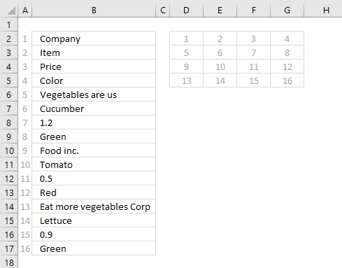
Combining the ROWS function and the COLUMNS function lets you build the number sequence shown above.
Formula in cell D2:
Explaining formula in cell D2

I almost always use the "Evaluate Formula" tool located on the Formulas tab on the ribbon. It allows me to see each calculation step the formula performs simply by pressing a button.
The underlined expression shows what part of the formula will be evaluated when you press with left mouse button on the "Evaluate" button. The italicized expression shows the most recent result of the evaluation.
Press with left mouse button on the "Evaluate button" to see the next step being calculated, keep press with left mouse button oning the "Evaluate" button and you will reach the final result. This can take quite some time if the formula has many steps to evaluate.
Step 1 - Calculate the number of columns in cell range
The COLUMNS function returns the number of columns in a given cell range. Cell reference $A$1:A1 contains both an absolute part $A$1 and a relative part A1 which makes the reference expanding when the cell is copied to adjacent cells.
COLUMNS($A$1:A1) returns 1.
Step 2 - Calculate the number of rows in cell range
The ROWS function returns the number of rows in a given cell range. Cell reference $A$1:A1 is also expanding when the cell is copied to adjacent cells.
ROWS($A$1:A1)*4
becomes
1*4
We need to multiply the result with 4 because we want to populate four columns. Change this value if you need a cell range with more or fewer columns.
1*4 returns 4.
Step 3 - Add numbers and subtract with 4
COLUMNS($A$1:A1)+ROWS($A$1:A1)*4-4
becomes
1+4-4
We need to subtract with four to make the first row zero. The next row will then evaluate to 4 and so on.
1+4-4 returns 1.
Step 4 - Get values
The INDEX function gets a value from cell range or array based on a row and column number, the column number is optional if you are working with a cell range that has only one column.
INDEX($B$2:$B$17, COLUMNS($A$1:A1)+ROWS($A$1:A1)*4-4)
becomes
INDEX($B$2:$B$17, 1)
and returns the value in cell B2 which is "Company".
Adjacent cells
Here is how the cell references change when the cell is copied to adjacent cells.
In cell D2 COLUMNS($A$1:A1) returns 1 and ROWS($A$1:A1)*4-4 returns 0 (zero). 1 +0 is 1. The INDEX function returns the first value in cell range B2:B17 which is "Company".
In cell E2 COLUMNS($A$1:A2) returns 2 and ROWS($A$1:A1)*4-4 returns 0 (zero). 2+0 is 2. The INDEX function returns the second value in cell range B2:B17 which is "Item".
In cell D3 COLUMNS($A$1:A1) returns 1 and ROWS($A$1:A2)*4-4 returns 4. 1+4 is 5. The INDEX function returns the fifth value in cell range B2:B17 which is "Vegetables are us".
2. Rearrange values from a single column cell range to a multicolumn cell range - Excel 365

This formula is a dynamic array formula that works only in Excel 365, it contains a new function namely the SEQUENCE function which can create a sequence of numbers.
Regular formula in cell D2:
=INDEX(B2:B17, SEQUENCE(4, 4))
2.1 Explaining formula in cell D2
Step 1 - Create a sequence from 1 to n
The SEQUENCE function creates a list of sequential numbers to a cell range or array.
SEQUENCE(rows, [columns], [start], [step])
The following setup returns an array of numbers from 1 to 16 split into four columns and four rows.
SEQUENCE(4,4)
returns
{1, 2, 3, 4; 5, 6, 7, 8; 9, 10, 11, 12; 13, 14, 15, 16}
The comma is a column delimiting character and the semicolon is a row delimiting character. This is based on your computer settings.

Step 2 - Get values from cell range B2:B17
The INDEX function returns a given value from a cell range based on a row and column number. The column number is optional.
INDEX(array, [row_num], [column_num])
INDEX(B2:B17,SEQUENCE(4,4))
becomes
INDEX(B2:B17, {1, 2, 3, 4; 5, 6, 7, 8; 9, 10, 11, 12; 13, 14, 15, 16})
becomes
INDEX({"Company"; "Item"; "Price"; "Color"; "Vegetables are us"; "Cucumber"; 1.2; "Green"; "Food inc."; "Tomato"; 0.5; "Red"; "Eat more vegetables Corp"; "Lettuce"; 0.9; "Green"}, {1, 2, 3, 4; 5, 6, 7, 8; 9, 10, 11, 12; 13, 14, 15, 16})
and returns
{"Company", "Item", "Price", "Color"; "Vegetables are us", "Cucumber", 1.2, "Green"; "Food inc.", "Tomato", 0.5, "Red"; "Eat more vegetables Corp", "Lettuce", 0.9, "Green"}.
3. Rearrange cell values from a single column to a multicolumn cell range

The image above demonstrates a formula that returns values from cell range D3:G5 to a single column, in this case, column B.
Formula in cell B2:
3.1 Explaining formula in cell B2
Step 1 to 3 calculates the first argument (row) in the INDEX function. Step 4 to 6 shows how to calculate the second argument (column) in the INDEX function.
INDEX function syntax: INDEX(array, row_num, [column_num])
Step 1 - Calculate rows in cell reference
The ROWS function returns the number of rows in a given cell range. Cell reference $A$1:A1 grows automatically when the cell is copied to adjacent cells.
The reason it is growing is that cell reference $A$1:A1 has an absolute and a relative part, read more here: Absolute and relative cell references
ROWS($A$1:A1)-1
becomes
1-1 and returns 0 (zero).
Step 2 - Calculate columns in the cell reference
The COLUMNS function returns the number of columns in a given cell reference.
COLUMNS($D$3:$G$5)
returns 4. (D, E, F, and G).
Step 3 - Divide first expression with the second expression
(ROWS($A$1:A1)-1)/COLUMNS($D$3:$G$5)
becomes
0/4
and returns 0 (zero).
Step 3 - Round the result down to the nearest whole number
The ROUNDDOWN function rounds a number down based on the number of digits specified in the second argument.
ROUNDDOWN(number, num_digits)
ROUNDDOWN((ROWS($A$1:A1)-1)/COLUMNS($D$3:$G$5),0)+1
becomes
ROUNDDOWN(0,0)+1
becomes
0 + 1
and returns 1.
Step 4 - Calculate rows in the cell reference
The ROWS function returns the number of rows in a given cell range. Cell reference $A$1:A1 grows when the cell is copied to cells below or to the right.
ROWS($A$1:A1)-1
becomes
1-1
and returns 0 (zero).
Step 5 - Calculate the number of columns in the cell reference
The COLUMNS function returns the number of columns in a given cell reference.
COLUMNS($D$3:$G$5)
returns 4 (D, E, F, and G).
Step 6 - Calculate reminder if the division
The MOD function returns the remainder after a number is divided by a divisor.
MOD(number, divisor)
MOD(ROWS($A$1:A1)-1,COLUMNS($D$3:$G$5))+1
becomes
MOD(1-1,COLUMNS($D$3:$G$5))+1
becomes
MOD(1-1,4)+1
becomes
MOD(0,4)+1
becomes
0+1
and returns 1.
Step 7 - Get value
The INDEX function gets a value from cell range or array based on a row and column number, the column number is optional if you are working with a cell range that has only one column.
INDEX($D$3:$G$5,ROUNDDOWN((ROWS($A$1:A1)-1)/COLUMNS($D$3:$G$5),0)+1, MOD(ROWS($A$1:A1)-1,COLUMNS($D$3:$G$5))+1)
becomes
INDEX($D$3:$G$5, 1, MOD(ROWS($A$1:A1)-1,COLUMNS($D$3:$G$5))+1)
becomes
INDEX($D$3:$G$5, 1, 1)
and returns "Vegetables are us" in cell B2.
5. Rearrange data

Sheet1A B C D
8 Country Europe
9 Lights 100
10 Type A 200
11
12 Country USA
13 Fuel 40
14 Diesel 200
15
16 Europe Lights Type A 100
17 USA Fuel Diesel 40
Oscar,is there a way to organize this the information into a database format like row 16 onwards,
It picks up all non blanks between the countries putting each line into a separate column.
This article describes two ways to rearrange data to rows based on an empty row as a delimiter. The first one uses the LAMBDA function to rearrange values, the second one demonstrates a User Defined Function that rearranges values.
Table of Contents
- Rearrange data - Excel 365 LAMBDA function
- Rearrange data - User defined function
5.1. Rearrange data - Excel 365 LAMBDA function
The image above demonstrates a LAMBDA function that rearranges values to single row. An empty row in the source data creates a new row of data in the result.
Excel 365 dynamic array formula:
This formula has a limit of 32767 characters, a result larger than that returns an error value.
Explaining formula
Step 1 - Join cell values
The TEXTJOIN function combines text strings from multiple cell ranges.
Function syntax: TEXTJOIN(delimiter, ignore_empty, text1, [text2], ...)
TEXTJOIN(",",1,a)
Step 2 - Build LAMBDA function
The LAMBDA function build custom functions without VBA, macros or javascript.
Function syntax: LAMBDA([parameter1, parameter2, …,] calculation)
LAMBDA(a,TEXTJOIN(",",1,a))
Step 3 - Perform calculation row by row
The BYROW function puts values from an array into a LAMBDA function row-wise.
Function syntax: BYROW(array, lambda(array, calculation))
BYROW(B2:D8,LAMBDA(a,TEXTJOIN(",",1,a)))
Step 4 - Check if value is empty
The IF function returns one value if the logical test is TRUE and another value if the logical test is FALSE.
Function syntax: IF(logical_test, [value_if_true], [value_if_false])
If value is empty a semicolon is appended to the accumulator value, if not a colon is attached.
IF(b="",a&";",a&","&b)
Step 5 - Build LAMBDA function
The LAMBDA function build custom functions without VBA, macros or javascript.
Function syntax: LAMBDA([parameter1, parameter2, …,] calculation)
LAMBDA(a,b,IF(b="",a&";",a&","&b))
Step 6 - Join values in the array
The REDUCE function shrinks an array to an accumulated value, a LAMBDA function is needed to properly accumulate each value in order to return a total.
Function syntax: REDUCE([initial_value], array, lambda(accumulator, value))
REDUCE(,BYROW(B2:D8,LAMBDA(a,TEXTJOIN(",",1,a))),LAMBDA(a,b,IF(b="",a&";",a&","&b)))
Step 7 - Split string based on semicolon and colon
The TEXTSPLIT function splits a string into an array based on delimiting values.
Function syntax: TEXTSPLIT(Input_Text, col_delimiter, [row_delimiter], [Ignore_Empty])
TEXTSPLIT(REDUCE(,BYROW(B2:D8,LAMBDA(a,TEXTJOIN(",",1,a))),LAMBDA(a,b,IF(b="",a&";",a&","&b))),",",";",TRUE)
5.2. Rearrange data - UDF

Answer:
I created a User Defined Function that rearranges non empty cells into rows, using a delimiting value. In the example below, "Country" is the delimiting value. The desired output is displayed in row 11 and 12 and the UDF is shown in row 15 and 16.
A User Defined Function is a custom function that anyone can use, simply copy the VBA code and paste to a code module in your workbook.
Array formula in cell A15:F17
How to enter array formula in cell range A15:F17
- Select cell range A15:F17.
- Type =OrganizeData("Country", A2:C8)
- Press and hold CTRL + SHIFT simultaneously.
- Press Enter once.
- Release all keys.
User defined Function Syntax
OrganizeData(srch, rng)
Arguments
| srch | Required. A delimiting value. |
| rng | Required. The range containing values you want to rearrange. |
VBA code
'Name User Defined Function
Function OrganizeData(srch As String, rng As Variant)

'Declare variables and data types
Dim cell As Range, temp() As Variant, ca As Single
Dim iRows As Integer, i As Integer, c As Single, r As Single
Dim chk As Boolean

'Make array temp as large as the cell range you entered the UDF in
ReDim temp(Range(Application.Caller.Address).Columns.Count - 1, 0)

'Save False to variable chk
chk = False

'Save values in cell range rng to array variable rng
rng = rng.Value

'Iterate through rows in rng variable
For r = LBound(rng, 1) To UBound(rng, 1)

    'Iterate through columns in array variable
    For c = LBound(rng, 2) To UBound(rng, 2)

        'If rng value is equal to delimiting value
        If rng(r, c) = srch Then

            'If Chk variable is not equal to False
            If chk <> False Then

                'Save blanks to temp variable based on value i
                For ca = i To UBound(temp, 1)
                    temp(ca, UBound(temp, 2)) = ""
                Next ca

                'Reset i to 0 (zero)
                i = 0

                'Increase array variable temp by 1
                ReDim Preserve temp(UBound(temp, 1), UBound(temp, 2) + 1)
            End If

            'Save True to variable chk
            chk = True

        'If rng variable is not equal to nothing and rng variable is not equal to delimiting value then
        ElseIf rng(r, c) <> "" And rng(r, c) <> srch Then

            'Save value to array variable temp
            temp(i, UBound(temp, 2)) = rng(r, c)

            'Increment i with 1
            i = i + 1
        End If
    Next c
Next r
'Save blanks to remaining values in array variable temp
For ca = i To UBound(temp, 1)
    temp(ca, UBound(temp, 2)) = ""
Next ca

'Increase containers in arrat variable temp with 1
ReDim Preserve temp(UBound(temp, 1), UBound(temp, 2) + 1)

'Count the number of rows you have entered the UDF in
iRows = Range(Application.Caller.Address).Rows.Count

'Save blanks to remaining cells
For r = UBound(temp, 2) To iRows
    For c = LBound(temp, 1) To UBound(temp, 1)
        temp(c, r) = ""
    Next c
    ReDim Preserve temp(UBound(temp, 1), UBound(temp, 2) + 1)
Next r

'Return values in temp to worksheet rearranged vertically
OrganizeData = Application.Transpose(temp)

End Function
Where to copy the code?
- Copy VBA code above.
- Press Alt+ F11 to open the Visual Basic Editor.
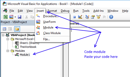
- Press with left mouse button on "Insert" on the top menu.
- Press with left mouse button on "Module" to create a module.
- Paste code to module
- Exit VBE and return to Excel
6. Rearrange values in a cell range to a single column
This section demonstrates formulas that rearrange values in a cell range to a single column.
Table of Contents
- Rearrange cells in a cell range to vertically distributed values (Excel formula)
- How to quickly create a named range
- Explaining array formula in cell B2
- Rearrange cells in a cell range to vertically distributed values (Excel 2019)
- Explaining array formula (Excel 2019)
- Returning values row by row
- Get Excel file
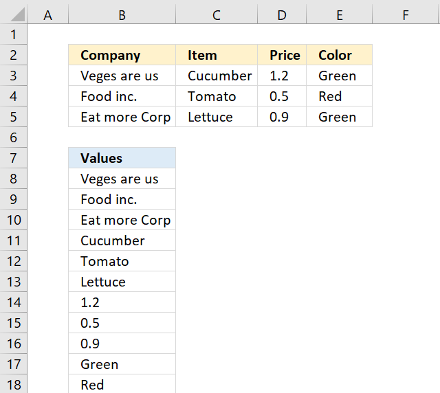
6.1. Rearrange cells in a cell range to vertically distributed values (Excel formula)
The formula in cell B8 uses a named range to calculate the row and column needed to extract the correct value.
rng is a named range and refers to cell range B3:E5.
Excel 365 dynamic array formula:
The TOCOL function is a newer function available to Excel 365 subscribers, it lets you rearrange values in a 2D cell range to a single column.
TOCOL(array, [ignore], [scan_by_col])
Use the following Excel 365 function to distribute values horizontally:
The TOROW function rearranges values from a 2D cell range to a single row.
TOROW(array, [ignore], [scan_by_col])
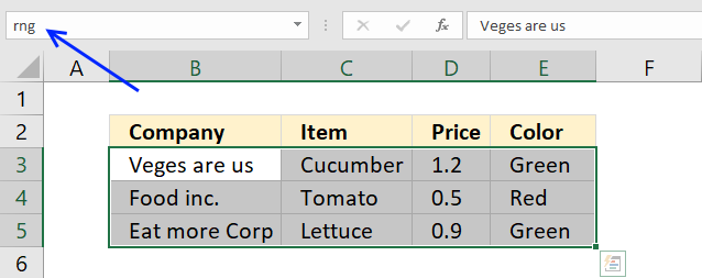
6.2. How to quickly create a named range
This step is optional, you can use just as well use a cell reference.
To create a named range simply select the cell range (B3:E5) and press with left mouse button on in the name box. Type a name for that range, I named the cell range rng. Press Enter, that's it.
6.3. Explaining formula in cell B8
Step 1 - Count rows in cell range
The INDEX function needs a row and column number in order to get the correct value.
The ROWS function returns the number of rows in a cell range.
ROWS(rng) becomes ROWS(B3:E5) and returns 3.
Step 2 - Create a sequence
The ROW function returns the row number of a cell reference.
ROW(A1) returns 1.
Step 3 - Create a repeating number sequence
To calculate the row number I use the MOD function to build a repeating number sequence. There are three rows in B3:E5 so the sequence must be 1,2,3,1,2,3, ... and so on.
MOD(ROW(A1)-1, ROWS(rng))+1
becomes
MOD(1-1, 3)+1
becomes
MOD(0, 3) + 1 and returns 1.
Step 4 - Create a repeating number sequence for columns
To calculate the column number I use the QUOTIENT function to build a repeating number sequence: 1,1,1,2,2,2,3 ... and so on.
QUOTIENT(ROW(A1)-1, ROWS(rng))+1
becomes
QUOTIENT(1-1, 3)+1
becomes
QUOTIENT(0, 3)+1 and returns 1.
Step 5 - Get value based on row and column numbers
The INDEX function then returns the value in row 1 and column 1 from cell range 3:E5.
INDEX(rng, MOD(ROW(A1)-1, ROWS(rng))+1, QUOTIENT(ROW(A1)-1, ROWS(rng))+1)
becomes
INDEX(rng, 1, 1)
and returns "Veges are us" in cell B8.
6.4. Rearrange cells in a cell range to vertically distributed values (Excel 2019 formula)

Array formula in cell B8:
Note, enter this formula as a regular formula if you are an Excel 365 user.
6.5. Explaining array formula (Excel 2019)
Step 1 - Join values using a delimiting character
The TEXTJOIN function joins values from a cell range or array, you need at least the Excel 2019 version.
TEXTJOIN(delimiter, ignore_empty, text1, [text2], ...)
I recommend using a delimiting character that is not in cell range B3:E5 to avoid confusion.
TEXTJOIN("|", TRUE, B3:E5)
becomes
TEXTJOIN("|",TRUE,{"Veges are us","Cucumber",1.2,"Green";"Food inc.","Tomato",0.5,"Red";"Eat more Corp","Lettuce",0.9,"Green"})
and returns
"Veges are us|Cucumber|1.2|Green|Food inc.|Tomato|0.5|Red|Eat more Corp|Lettuce|0.9|Green"
Step 2 - Substitute delimiting character with XML tag
The SUBSTITUTE function substitutes a specific text string in a value.
SUBSTITUTE(text, old_text, new_text, [instance_num])
SUBSTITUTE(TEXTJOIN("|", TRUE, B3:E5), "|","</B><B>")
becomes
SUBSTITUTE("Veges are us|Cucumber|1.2|Green|Food inc.|Tomato|0.5|Red|Eat more Corp|Lettuce|0.9|Green", "|","</B><B>")
and returns
"Veges are us</B><B>Cucumber</B><B>1.2</B><B>Green</B><B>Food inc.</B><B>Tomato</B><B>0.5</B><B>Red</B><B>Eat more Corp</B><B>Lettuce</B><B>0.9</B><B>Green"
Step 3 - Concatenate string with XML tag
The ampersand character & lets you concatenate strings in an Excel formula.
"<A><B>"&SUBSTITUTE("Veges are us|Cucumber|1.2|Green|Food inc.|Tomato|0.5|Red|Eat more Corp|Lettuce|0.9|Green", "|","</B><B>")&"</B></A>"
becomes
"<A><B>"&"Veges are us</B><B>Cucumber</B><B>1.2</B><B>Green</B><B>Food inc.</B><B>Tomato</B><B>0.5</B><B>Red</B><B>Eat more Corp</B><B>Lettuce</B><B>0.9</B><B>Green"&"</B></A>"
and returns
"<A><B>Veges are us</B><B>Cucumber</B><B>1.2</B><B>Green</B><B>Food inc.</B><B>Tomato</B><B>0.5</B><B>Red</B><B>Eat more Corp</B><B>Lettuce</B><B>0.9</B><B>Green</B></A>"
Step 4 - Extract values from XML data
The FILTERXML function extracts specific values from XML content by using the given xpath.
FILTERXML(xml, xpath)
FILTERXML("<A><B>"&SUBSTITUTE(TEXTJOIN("|", TRUE, B3:E5), "|","</B><B>")&"</B></A>","//B")
becomes
FILTERXML("<A><B>Veges are us</B><B>Cucumber</B><B>1.2</B><B>Green</B><B>Food inc.</B><B>Tomato</B><B>0.5</B><B>Red</B><B>Eat more Corp</B><B>Lettuce</B><B>0.9</B><B>Green</B></A>","//B")
and returns
{"Veges are us"; "Cucumber"; 1.2; "Green"; "Food inc."; "Tomato"; 0.5; "Red"; "Eat more Corp"; "Lettuce"; 0.9; "Green"}.
6.6. Returning values row by row
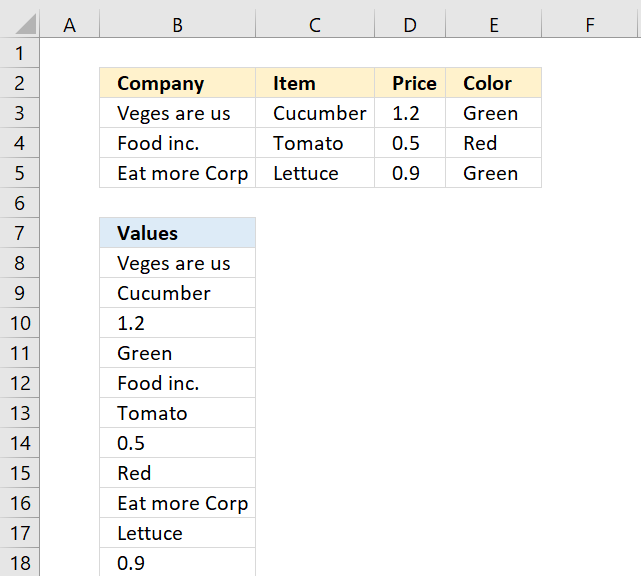
The following formula gets the values row by row:
Excel 365 dynamic array formula:
The TOCOL function is a newer function available to Excel 365 subscribers, it lets you rearrange values in a 2D cell range to a single column.
TOCOL(array, [ignore], [scan_by_col])
7. Resize a range of values - UDF

The User Defined Function (UDF) demonstrated in this section resizes a given range to columns or rows you specify.
The image above shows the UDF entered in cell range G3:J6 as an array formula, it takes the values in column D and rearranges them into four columns and as many rows as needed.
What's on this section
- ResizeRange function (User Defined Function)
- VBA Code
- Where do I put the code?
- Explaining the User Defined Function (UDF)
- Get Excel file
7.1. ResizeRange function
The first argument is the range, the second argument is how many columns you want and the third argument is how many rows you want in your new range.
UDF Syntax
Arguments
range - cell range you want to resize
rows - the number of rows you want, leave it to 0 (zero) if you want the udf to calculate the number of rows needed
columns - the number of columns you want, leave it to 0 (zero) if you want the udf to calculate the number of columns needed.
The picture above shows values in column c, C2:C17 being resized into a range of 4 columns. The User Defined Function calculates the number of rows that are needed, to do that use 0 (zero) as the row argument:
If you want 2 rows and as many columns as needed the UDF becomes:
7.2. VBA Code
'Name User Defined Function and dimension parameters
Function ResizeRange(rng As Range, r As Single, c As Single)

'Dimension variables and declare their data types
Dim rngV As Variant
Dim tbl() As Variant
Dim Value As Variant

'Save values from range object rng to array variable rngV
rngV = rng.Value

'If ... Then ... Else ... Endif statement
If r = 0 Then

'Count cells in range object rng and divide by value in variable c, then round up to a whole number and save to variable r
r = Application.WorksheetFunction.RoundUp(rng.Cells.CountLarge / c, 0)

'Continue here if variable c is 0 (zero)
ElseIf c = 0 Then

'Count cells in range object rng and divide by value in variable r, then round up to a whole number and save to variable c
c = Application.WorksheetFunction.RoundUp(rng.Cells.CountLarge / r, 0)
End If

'Redimension array variable tbl based on variables c and r
ReDim tbl(1 To r, 1 To c)

'Save 1 to variable r
r = 1

'Save 0 (zero) to variable c
c = 0

'Transpose values in variable rngV and save to variable rngV
rngV = Application.Transpose(rngV)

'For each statement
For Each Value In rngV

'If .. Endif statement
'Check if c is equal to the number of columns in array variable tbl
If c = UBound(tbl, 2) Then

'Add 1 to the value stored in array variable r and save to variable r
r = r + 1

'Save 0 (zero) to variable c
c = 0
End If

'Add 1 to the value stored in array variable c and save to variable c
c = c + 1

'Save value in variable Value to array variable tbl
tbl(r, c) = Value

'Continue with next value
Next Value

'Return values to worksheet
ResizeRange = tbl
End Function
7.3. Where do I put the code?
Copy the code above to a module:
How to insert a module to a workbook.
Go back to Excel from VB Editor.
Select a cell range, type the udf and it's arguments. See animated picture at the beginning of this post.
Create an array formula, here are the details if you don't know how to.
- Press and hold CTRL + SHIFT simultaneously
- Press Enter
- Release all keys
If you did it right the formula now has a curly bracket before and after. Like this {=ResizeRange(C2:C17, 2, 0)}. Don't enter these characters yourself.
7.4. Explaining the User Defined Function (UDF)
Function name and arguments
A user defined function always starts with "Function" and then a name. This udf has a three arguments. Variable rng is a range object, r and c are declared as Single. Read more about Defining data types.
Function ResizeRange(rng As Range, r As Single, c As Single)
Declaring variables
Value, tbl and rngV are all variants. tbl has two parenthesis meaning it is an array. Read more about Defining data types.
Dim rngV As Variant
Dim tbl() As Variant
Dim Value As Variant
Convert values from rng (range object) to rngV (variant array)
This speeds up the function considerably if you are working with large cell ranges. Excel copies all the values from the sheet and puts them in memory (array).
rngV = rng.Value
If ... then... ElseIf ... End If
Checks if r equals to 0 (zero) and if true then calculates needed rows. Checks also if c equals to 0 (zero) and then if true calculates needed columns.
If r = 0 Then
r = Application.WorksheetFunction.RoundUp(rng.Cells.CountLarge / c, 0)
ElseIf c = 0 Then
c = Application.WorksheetFunction.RoundUp(rng.Cells.CountLarge / r, 0)
End If
Build array
Now we know how many columns and rows we need to build the array. ReDim changes the array size.
ReDim tbl(1 To r, 1 To c)
Use variables r and c to save values in array
I am reusing these variables to help me know where to put each rngV value in tbl array. r is equal to 1 and c is equal to 0 (zero).
r = 1
c = 0
Transpose array
An array with 2 rows and 4 columns becomes an array with 4 rows and 2 columns, read more about transposing an array or range.
rngV = Application.Transpose(rngV)
For ... Next statement
Repeats a group of statements a specified number of times.
For Each Value In rngV
Next Value
If ... then... End If
Checks if c is equal to the number of columns in tbl array then, if true, adds 1 to r and c is equal to 0 (zero)
If c = UBound(tbl, 2) Then
r = r + 1
c = 0
End If
Add 1 to variable c
c is equal to c + 1
c = c + 1
Save value to tbl array
r is the row number and c is the column number in tbl array.
tbl(r, c) = Value
Return tbl array values to function
The ResizeRange returns an array of values stored in tbl.
ResizeRange = tbl
End a udf
A function procedure ends with this statement.
End Function
Rearrange values category
More than 1300 Excel formulasExcel categories
Leave a Reply
How to comment
How to add a formula to your comment
<code>Insert your formula here.</code>
Convert less than and larger than signs
Use html character entities instead of less than and larger than signs.
< becomes < and > becomes >
How to add VBA code to your comment
[vb 1="vbnet" language=","]
Put your VBA code here.
[/vb]
How to add a picture to your comment:
Upload picture to postimage.org or imgur
Paste image link to your comment.