How to use the MOD function

What is the MOD function?

The Mod function returns the remainder after a number is divided by a divisor. The Mod function is short for the Modulo operation (wikipedia).

The image above shows that the remainder of 11/2 is 1. 5*2 = 10. 11-10 = 1.

1. Introduction

What is the Modulo operation?

The modulo operation gives the remainder. Example, for an equation like 10 modulo 3:

10 is divided by 3 as much as possible, 3 goes into 10 3 times (divisor is 3). The remainder left over is 1, so 10 modulo 3 = 1

What is a remainder?

The remainder is what is left over after division of one number by another.

12 /5 = 2 and the remainder is 2. 2*5 = 10 + 2 = 12

What is a division?

Division is one of the four basic operations of arithmetic. It refers to the operation of determining how many times one number (the divisor) is contained within another number (the dividend).

It splits a quantity into equal groups or subsets. The result is called the quotient. Any amount left over is the remainder.

What is a divisor?

A divisor is a number that divides into another number either cleanly or leaving a remainder.

dividend / divisor = quotient( + remainder)

2. Syntax

MOD(number, divisor)

3. Example 1

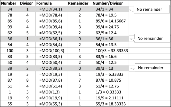
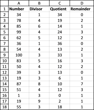
The image above demonstrates the result the MOD function returns using different numbers in both arguments number and divisor. The MOD function is in column "Remainder".

1. The first number is 34 and the divisor is 1. 34/1 equals 34 with 0 (zero) remainders.
2. The second number is 78, the divisor is 4. 78/4 = 19.5 There remainder is 2. 4*19 = 76. 78 - 76 = 2
3. The third number is 85, the divisor is 6. 85/6 equals approx. 14.16667. The remainder is 1. 14*6 = 84. 85-84 = 1
4. The fourth number is 99 and the divisor is 4. 99/4 = 24.75. The remainder is 3. 24*4 = 96. 99 - 96 = 3
5. The fifth number is 62 and the divisor is 5. 62/5 = 12.4. 12*5 = 60 62-60 = 2 The remainder is 2.

Back to top

4. Example 2

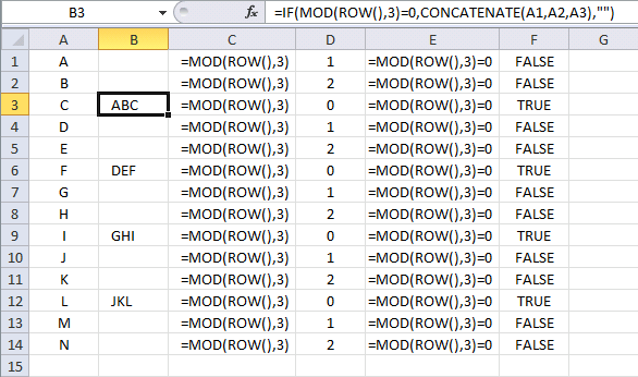
This example demonstrates a formula that joins the three last cell values every third row. The following formula concatenates cells in column A every third row:

Lets begin with ROW() in cell B3. It is dynamic and changes for each row. It returns the current row number, example in cell B3 ROW() returns 3.

Then the MOD function takes 3 and divides it with 3. MOD(ROW(), 3) returns 0.  The remainder is zero in cell B3. You can see this part of the formula in column C and the result in column D.

MOD(ROW(),3)=0 is a logical expression, it checks if the result from the MOD function is equal to 0 (zero). In every third row it is equal and returns TRUE, MOD(ROW(),3)=0 returns TRUE. You can see this part of the formula in column E and the result in column F.

The IF function returns CONCATENATE(A1, A2, A3) if the logical expression is TRUE or a blank if the logical expression is FALSE.

There are relative cell references in the CONCATENATE function and they change in each cell. Don't know much about relative and absolute cell references? Read this: Absolute and relative references in excel

Back to top

5. Example 3

This example demonstrates how to highlight every n-th row using the MOD function. You can use the same technique to highlight every second row with conditional formatting.

Here is how to apply conditional formatting to a cell range:

• Select a cell range.
• Go to the "Home" tab on the ribbon.
• Press with left mouse button on the Conditional formatting button.
• Press with left mouse button on "New Rule...".
• Press with left mouse button on "Use a formula to determine which cells to format:".
  
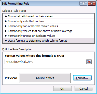
• Type the formula below. Press with left mouse button on the "Format" button. Go to tab "Fill". Pick a color. Press with left mouse button on OK twice.

Conditional formatting formula:

If you want to highlight every third row change the formula to =MOD(ROW(A1),3)=0.

Tip! Use Excel Tables to automatically format every other row if you don't want to use formulas and Conditional Formatting. You can easily change the formatting, select any cell in the Excel Table. A new tab appears on the ribbon named "Table Desing".Press with mouse on tab "Table Design". Press with mouse on any table style to quickly change formatting.

Back to top

6. Example 4

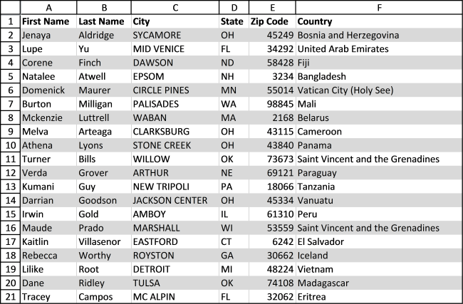
This conditional formatting rule highlights every other group based on values in column B. Column B must be sorted.

Conditional formatting formula:

Explaining CF formula in cell B3

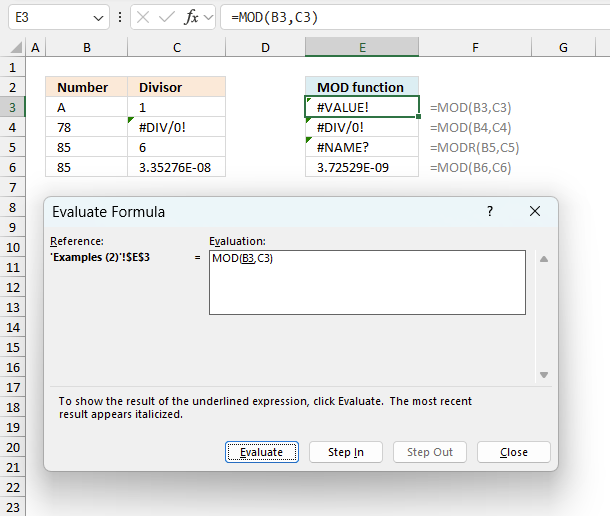
I recommend that you enter the formula in cell F3 to be able to evaluate the formula using the "Evaluate Formula" tool. The formula returns either TRUE or FALSE and the row is highlighted if it returns TRUE.

To start the "Evaluate Formula" tool go to tab "Formulas" on the ribbon.  Press with left mouse button on the "Evaluate Formula" button and a dialog box shows up.

Step 1 - Count cells based on a condition or criteria

The COUNTIF function calculates the number of cells that is equal to a condition.

COUNTIF(range, criteria)

Note that the cell references expand when the cell is copied to the cells below. In this case, the formula is used apply "Conditional Formatting" and the cell references changes depending on which cell is evaluated.

COUNTIF($B$2:$B2,$B$2:$B2)

becomes

COUNTIF("A1","A1")

and returns 1.

Step 2 - Divide 1 with the result

1/COUNTIF($B$2:$B2,$B$2:$B2)

becomes

1/1

and returns 1.

Step 3 - Sum array

The SUM function adds the numbers in a cell range or array and returns a total.

SUM(1/COUNTIF($B$2:$B2,$B$2:$B2))

becomes

SUM(1)

and returns 1.

Step 4 - Divide total with 2 and calculate remainder

MOD(SUM(1/COUNTIF($B$2:$B2,$B$2:$B2)),2)

becomes

MOD(1, 2)

and returns 1. 1 is equal to boolean value TRUE, cell B3 is highlighted.

Back to top

7. Example 5

This example demonstrates how to highlight groups based on values in all three columns: B, C and D. These values are evaluated per row meaning values in column B, C, and D forms a group based on each row.

Conditional formatting formula:

Make sure you get the relative and absolute cell references right.

Explaining CF formula

Step 1 - Count equal rows

The COUNTIFS function calculates the number of cells across multiple ranges that equals all given conditions.

The cell references $B$2:$B2 and so on expands automatically when the CF applies the conditional formatting formula to cells below. This makes the formula remember previous rows and is able to highlight correct rows.

COUNTIFS(criteria_range1, criteria1, [criteria_range2, criteria2]…)

COUNTIFS($B$2:$B2, $B$2:$B2, $C$2:$C2, $C$2:$C2, $D$2:$D2, $D$2:$D2)

becomes

COUNTIFS(1, 1, "A1", "A1", "AA", "AA")

and returns 1.

Step 2 - Divide 1 with result

1/COUNTIFS($B$2:$B2, $B$2:$B2, $C$2:$C2, $C$2:$C2, $D$2:$D2, $D$2:$D2)

becomes

1/1

and returns 1.

Step 3 - Sum numbers

The SUM function adds the numbers in a cell range or array and returns a total.

SUM(1/COUNTIFS($B$2:$B2, $B$2:$B2, $C$2:$C2, $C$2:$C2, $D$2:$D2, $D$2:$D2)

becomes

SUM(1)

and returns 1.

Step 4 - Calculate remainder

MOD(SUM(1/COUNTIFS($B$2:$B2, $B$2:$B2, $C$2:$C2, $C$2:$C2, $D$2:$D2, $D$2:$D2), 2)

becomes

MOD(1,2)

and returns 1.

Back to top

8. Example 6

How to return the fractional part of a number?
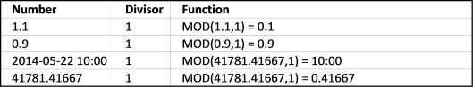
If you use 1 as a divisor the MOD function returns only the fraction of a number, in other words, only the decimals.
number - INT(number/divisor)

You can use this technique to return the time part from a cell containing date and time, see row 3 in the picture above.

Back to top

9. Example 7

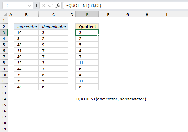
How to calculate the integer portion of a division?
The QUOTIENT function returns a number without the fractional component. 78 / 4 = 19.5
The quotient is 19. Here are more examples, the quotients are in column C.
QUOTIENT(numerator, denominator) uses the same arguments as the MOD function.

Back to top

10. Example 8

How to remove whole number and return decimal?
The formula in cell C3 removes the whole number and returns only the decimal part.

Formula in cell C3:

The formula above won't work with negative numbers, see cell C6 above. This formula in cell C3 works with both positive and negative numbers:

Explaining formula in cell C6

Step 1 - Logical test

B3<0 becomes -1.2<0 returns TRUE.

Step 2 - Evaluate TRUE argument in IF function

The IF function returns one value if the logical test is TRUE and another value if the logical test is FALSE.

Function syntax: IF(logical_test, [value_if_true], [value_if_false])

Step 3 - Convert negative value to positive

The ABS function converts negative numbers to positive numbers.

Function syntax: ABS(number)

ABS(B3) becomes ABS(-1.2) returns 1.2

Step 4 - Convert negative value to positive

MOD(ABS(B3), 1) becomes MOD(1.2, 1) and returns 0.2

Step 5 - Convert positive value to negative

-MOD(ABS(B3), 1) returns -1.2

Back to top

11. Function not working

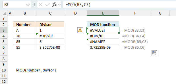
The MOD function returns

• #VALUE! error if you use a non-numeric input value.
• #NAME? error if you misspell the function name.
• propagates errors, meaning that if the input contains an error (e.g., #VALUE!, #REF!), the function will return the same error.

There seems to be a problem with large numbers and Microsoft knows about it:
https://support.microsoft.com/kb/119083

The MOD() function returns the #NUM! error if the following condition is true:
('divisor' * 134217728) is less than or equal to 'number'

This error seems to have been solved in Excel 365.

11.1 Troubleshooting the error value

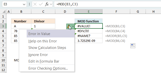
When you encounter an error value in a cell a warning symbol appears, displayed in the image above. Press with mouse on it to see a pop-up menu that lets you get more information about the error.

1. The first line describes the error if you press with left mouse button on it.
2. The second line opens a pane that explains the error in greater detail.
3. The third line takes you to the "Evaluate Formula" tool, a dialog box appears allowing you to examine the formula in greater detail.
4. This line lets you ignore the error value meaning the warning icon disappears, however, the error is still in the cell.
5. The fifth line lets you edit the formula in the Formula bar.
6. The sixth line opens the Excel settings so you can adjust the Error Checking Options.

Here are a few of the most common Excel errors you may encounter.

#NULL error - This error occurs most often if you by mistake use a space character in a formula where it shouldn't be. Excel interprets a space character as an intersection operator. If the ranges don't intersect an #NULL error is returned. The #NULL! error occurs when a formula attempts to calculate the intersection of two ranges that do not actually intersect. This can happen when the wrong range operator is used in the formula, or when the intersection operator (represented by a space character) is used between two ranges that do not overlap. To fix this error double check that the ranges referenced in the formula that use the intersection operator actually have cells in common.

#SPILL error - The #SPILL! error occurs only in version Excel 365 and is caused by a dynamic array being to large, meaning there are cells below and/or to the right that are not empty. This prevents the dynamic array formula expanding into new empty cells.

#DIV/0 error - This error happens if you try to divide a number by 0 (zero) or a value that equates to zero which is not possible mathematically.

#VALUE error - The #VALUE error occurs when a formula has a value that is of the wrong data type. Such as text where a number is expected or when dates are evaluated as text.

#REF error - The #REF error happens when a cell reference is invalid. This can happen if a cell is deleted that is referenced by a formula.

#NAME error - The #NAME error happens if you misspelled a function or a named range.

#NUM error - The #NUM error shows up when you try to use invalid numeric values in formulas, like square root of a negative number.

#N/A error - The #N/A error happens when a value is not available for a formula or found in a given cell range, for example in the VLOOKUP or MATCH functions.

#GETTING_DATA error - The #GETTING_DATA error shows while external sources are loading, this can indicate a delay in fetching the data or that the external source is unavailable right now.

11.2 The formula returns an unexpected value

To understand why a formula returns an unexpected value we need to examine the calculations steps in detail. Luckily, Excel has a tool that is really handy in these situations. Here is how to troubleshoot a formula:

1. Select the cell containing the formula you want to examine in detail.
2. Go to tab “Formulas” on the ribbon.
3. Press with left mouse button on "Evaluate Formula" button. A dialog box appears.
   The formula appears in a white field inside the dialog box. Underlined expressions are calculations being processed in the next step. The italicized expression is the most recent result. The buttons at the bottom of the dialog box allows you to evaluate the formula in smaller calculations which you control.
4. Press with left mouse button on the "Evaluate" button located at the bottom of the dialog box to process the underlined expression.
5. Repeat pressing the "Evaluate" button until you have seen all calculations step by step. This allows you to examine the formula in greater detail and hopefully find the culprit.
6. Press "Close" button to dismiss the dialog box.

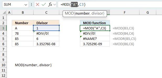
There is also another way to debug formulas using the function key F9. F9 is especially useful if you have a feeling that a specific part of the formula is the issue, this makes it faster than the "Evaluate Formula" tool since you don't need to go through all calculations to find the issue..

1. Enter Edit mode: Double-press with left mouse button on the cell or press F2 to enter Edit mode for the formula.
2. Select part of the formula: Highlight the specific part of the formula you want to evaluate. You can select and evaluate any part of the formula that could work as a standalone formula.
3. Press F9: This will calculate and display the result of just that selected portion.
4. Evaluate step-by-step: You can select and evaluate different parts of the formula to see intermediate results.
5. Check for errors: This allows you to pinpoint which part of a complex formula may be causing an error.

The image above shows cell reference B3 converted to hard-coded value using the F9 key. The MOD function requires numerical values which is not the case in this example. We have found what is wrong with the formula.

Tips!

• View actual values: Selecting a cell reference and pressing F9 will show the actual values in those cells.
• Exit safely: Press Esc to exit Edit mode without changing the formula. Don't press Enter, as that would replace the formula part with the calculated value.
• Full recalculation: Pressing F9 outside of Edit mode will recalculate all formulas in the workbook.

Remember to be careful not to accidentally overwrite parts of your formula when using F9. Always exit with Esc rather than Enter to preserve the original formula. However, if you make a mistake overwriting the formula it is not the end of the world. You can “undo” the action by pressing keyboard shortcut keys CTRL + z or pressing the “Undo” button

11.3 Other errors

Floating-point arithmetic may give inaccurate results in Excel - Article

Floating-point errors are usually very small, often beyond the 15th decimal place, and in most cases don't affect calculations significantly.

Back to top

Get the Excel file

How-to-use-the-MOD-function.xlsx

Useful links

MOD Function - Microsoft
Extracting Vectors From A Matrix

Back to top

'MOD' function examples

How to create date ranges in Excel
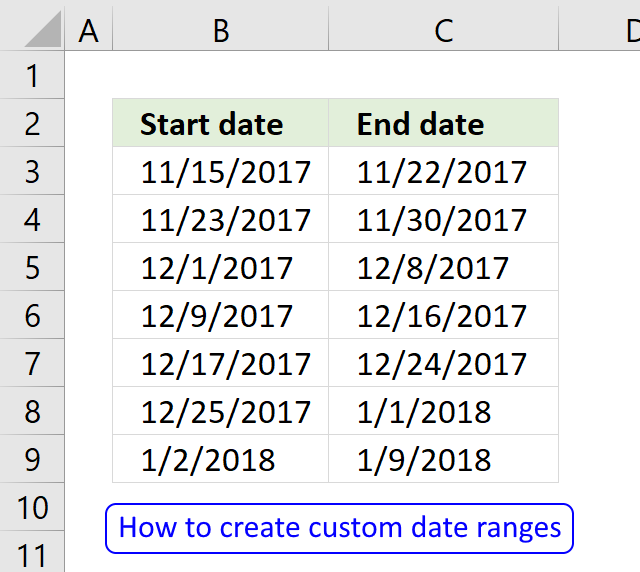
Question: I am trying to create an excel spreadsheet that has a date range. Example: Cell A1 1/4/2009-1/10/2009 Cell B1 […]

Find numbers closest to sum
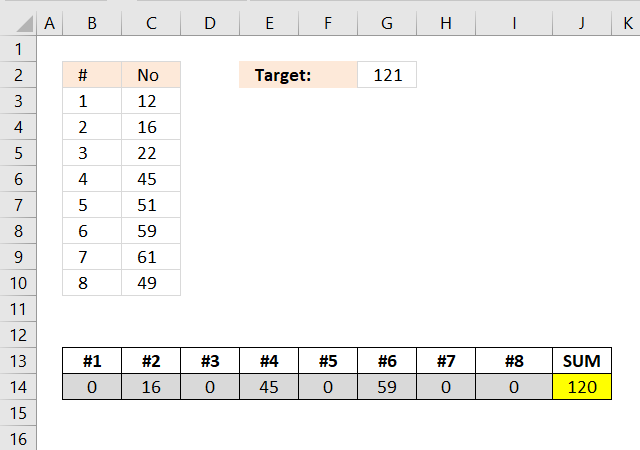
Excelxor is such a great website for inspiration, I am really impressed by this post Which numbers add up to […]

How to create permutations
I discussed the difference between permutations and combinations in my last post, today I want to talk about two kinds […]

'MOD' function examples

How to use the QUOTIENT function
The quotient function returns the integer portion of a division. The remainder is left out. This function is useful in […]

Rearrange values using formulas
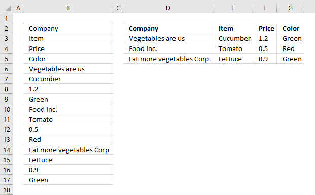
The picture above shows data presented in only one column (column B), this happens sometimes when you get an undesired […]

Functions in 'Math and trigonometry' category

The MOD function function is one of 62 functions in the 'Math and trigonometry' category.

Excel categories

Comments (8)