How to use the QUOTIENT function

The quotient function returns the integer portion of a division. The remainder is left out. This function is useful in scenarios where you need only the whole number result of a division, ignoring any fractional part.
Example, 5/2 = 2.5. The integer is 2. The remainder is 0.5
What's on this webpage
1. Introduction
What is an integer?
An integer is a whole number that can be positive, negative, or zero, but not a fraction or decimal.
What is a whole number?
A whole number is a number without any fractional or decimal parts. Whole numbers are the set of non-negative integers. Examples: 0, 1, 2, 3, 4, 5, and so on.
Whole numbers are used for counting discrete objects and in many basic mathematical operations. While whole numbers include only non-negative integers, the set of integers includes negative numbers as well.
What is a remainder?
A remainder is what's left over after division when one number doesn't divide evenly into another. The amount left over when one number cannot be divided evenly by another.
In the division 17 ÷ 5 The quotient is 3. The remainder is 2 (Because 5 goes into 17 three times with 2 left over)
What is division?
Division in mathematics is one of the four basic arithmetic operations, alongside addition, subtraction, and multiplication. Division is the process of splitting a quantity into equal parts or groups.
Components:
- Dividend: The number being divided
- Divisor: The number dividing the dividend
- Quotient: The result of the division
- Remainder: The amount left over (if division isn't exact)
Example:
- In 20 ÷ 4 = 5
- 20 is the dividend
- 4 is the divisor
- 5 is the quotient
Types:
- Exact division: No remainder (e.g., 12 ÷ 3 = 4)
- Non-exact division: Has a remainder (e.g., 14 ÷ 3 = 4 remainder 2)
2. Syntax
QUOTIENT(numerator, denominator)
| numerator | Required. The dividend. |
| denominator | Required. The divisor. |
The QUOTIENT function returns the #VALUE! if the arguments are not numbers.
The following formula is equivalent to the QUOTIENT function:
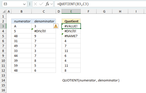
3. Example 1
The first example uses 10 as the numerator and 3 as the denominator located in cells B3 and C3 respectively. The QUOTIENT function output in cell E3 is 3.
Formula in cell E3:
Lets do some manual calculations, what is the integer part of 10 divided by 3?
10 / 3 = 3.333333 The integer part is 3.
3 * 3 = 9
10 - 9 = 1 The remainder is 1.
The second example uses 5 as the numerator and 2 as the denominator located in cells B4 and C4 respectively. The QUOTIENT function output in cell E4 is 2.
Formula in cell E4:
Lets do some manual calculations, what is the integer part of 5 divided by 2?
5 / 2 = 2.5 The integer part is 2.
2 * 2 = 5
5 - 4 = 1 The remainder is 1.
The third example uses 48 as the numerator and 9 as the denominator located in cells B5 and C5 respectively. The QUOTIENT function output in cell E5 is 5.
Formula in cell E5:
Lets do some manual calculations, what is the integer part of 48 divided by 9?
48 / 9 = 5 The integer part is 5.
9 * 5 = 45
48 - 45 = 3 The remainder is 3.
4. Example 2

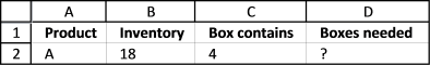
You're preparing to ship your company's products to customers. You have:
- 18 units of product A in stock (stored in cell B2)
- Shipping boxes that can each hold 4 units of product A (capacity stored in cell C2)
How many boxes will you need to package product A for shipping if all boxes needs to be full?
QUOTIENT(numerator, denominator)
There are two arguments, the numerator is the dividend and the denominator is the divisor.
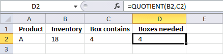
The formula in cell D2:
returns 4. This means that you need 4 boxes to ship 16 products. 2 products remains.
If you divide 18 by 4, you get 4.5.
The Quotient function returns 4 because the integer part of 4.5 is 4.
5. Example 3

How to find divisors of a number that return no remainders?
The formula in cell C4 shown in the image above is a dynamic array formula that automatically spills values to cells below. It calculates all divisors that can be used so the result returns a whole number based on the dividend specified in cell C2.
Example, number 5 returns no remainders. 100/5 = 20. The result is a whole number. Change the number in cell C2 and Excel automatically calculates divisors in cell C4 and cells below. There is a dividend limit of 1048576, you can't go higher than that.
Excel 365 formula in cell C4:
The following formula is an array formula, it works for all previous Excel versions and returns the same numbers as the Excel 365 formula.
Array formula for previous Excel versions:
How to enter an array formula
- Double press with left mouse button on with left mouse button on cell C4.
- Paste the formula.
- Press and hold CTRL + SHIFT keys simultaneously.
- Press Enter once.
- Release all keys.
Copy cell C4 and paste to cells below as far as needed. This is required if you are using the array formula.
Explaining Excel 365 formula in cell C4
Step 1 - Create a sequence
The SEQUENCE function returns an array containing a sequence of numbers.
SEQUENCE(C2)
becomes
SEQUENCE(100)
and returns {1; 2; 3; ... 98; 99; 100}. Not all numbers are shown in this sequence.
Step 2 - Calculate remainders
The MOD function returns the remainder of a division.
MOD($C$2,SEQUENCE($C$2))
becomes
MOD(100, {1; 2; 3; ... 98; 99; 100})
and returns {0 ;0 ;1 ; ... ; 2; 1; 0}.
Step 3 - Create a logical expression
The equal sign allows you to compare the numbers in the array to 0 (zero). The result is boolean values TRUE or FALSE.
MOD(C2,SEQUENCE(C2))=0
becomes
{0 ;0 ;1 ; ... ; 2; 1; 0}=0
and returns {TRUE ;TRUE ;FALSE; ... ; FALSE; FALSE; TRUE }.
Step 4 - Filter values based on logical expression
The FILTER function lets you extract values/rows based on a condition or criteria.
FILTER(SEQUENCE(C2), MOD(C2,SEQUENCE(C2))=0)
becomes
FILTER(SEQUENCE(C2), {TRUE ;TRUE ;FALSE; ... ; FALSE; FALSE; TRUE })
becomes
FILTER({1; 2; 3; ... 98; 99; 100}, {TRUE ;TRUE ;FALSE; ... ; FALSE; FALSE; TRUE })
and returns {1; 2; 4; 5; 10; 20; 25; 50; 100}.
6. Example 4

The image above demonstrates a formula that returns repeating numbers in a sequence. For example, 0, 0, 0, 1, 1, 1, 2, 2, 2 etc.
The second argument determines how many times a number is repeated before moving on to the next number.
Formula in cell B3:
Change the formula to this if you want the sequence to start with 1 instead of 0 (zero).
Explaining formula in cell B3
Step 1 - Calculate a number that changes based on a relative and absolute cell ref
The ROWS function returns a number representing the number of rows in cell reference. Cell ref $A$1:A1 is a growing cell reference that changes when you copy the cell and paste to cells below.
It contains an absolute ($A$1) indicated by the dollar signs and a relative part (A1).
ROWS($A$1:A1)-1
becomes
1-1
amd returns 0 (zero).
Step 2 - Calculate quotient
QUOTIENT(numerator, denominator)
QUOTIENT(ROWS($A$1:A1)-1,3)
becomes
QUOTIENT(0,3)
and returns 0 (zero) in cell B3.
7. Function not working
The QUOTIENT function returns
- #VALUE! error if you use a non-numeric input value.
- #NAME? error if you misspell the function name.
- propagates errors, meaning that if the input contains an error (e.g., #VALUE!, #REF!), the function will return the same error.
7.1 Troubleshooting the error value
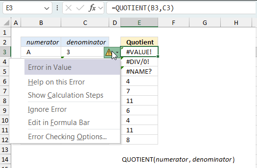
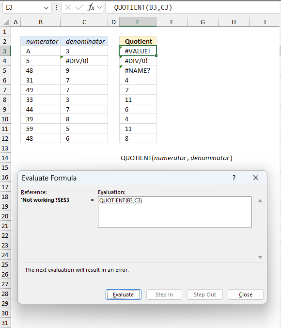
When you encounter an error value in a cell a warning symbol appears, displayed in the image above. Press with mouse on it to see a pop-up menu that lets you get more information about the error.
- The first line describes the error if you press with left mouse button on it.
- The second line opens a pane that explains the error in greater detail.
- The third line takes you to the "Evaluate Formula" tool, a dialog box appears allowing you to examine the formula in greater detail.
- This line lets you ignore the error value meaning the warning icon disappears, however, the error is still in the cell.
- The fifth line lets you edit the formula in the Formula bar.
- The sixth line opens the Excel settings so you can adjust the Error Checking Options.
Here are a few of the most common Excel errors you may encounter.
#NULL error - This error occurs most often if you by mistake use a space character in a formula where it shouldn't be. Excel interprets a space character as an intersection operator. If the ranges don't intersect an #NULL error is returned. The #NULL! error occurs when a formula attempts to calculate the intersection of two ranges that do not actually intersect. This can happen when the wrong range operator is used in the formula, or when the intersection operator (represented by a space character) is used between two ranges that do not overlap. To fix this error double check that the ranges referenced in the formula that use the intersection operator actually have cells in common.
#SPILL error - The #SPILL! error occurs only in version Excel 365 and is caused by a dynamic array being to large, meaning there are cells below and/or to the right that are not empty. This prevents the dynamic array formula expanding into new empty cells.
#DIV/0 error - This error happens if you try to divide a number by 0 (zero) or a value that equates to zero which is not possible mathematically.
#VALUE error - The #VALUE error occurs when a formula has a value that is of the wrong data type. Such as text where a number is expected or when dates are evaluated as text.
#REF error - The #REF error happens when a cell reference is invalid. This can happen if a cell is deleted that is referenced by a formula.
#NAME error - The #NAME error happens if you misspelled a function or a named range.
#NUM error - The #NUM error shows up when you try to use invalid numeric values in formulas, like square root of a negative number.
#N/A error - The #N/A error happens when a value is not available for a formula or found in a given cell range, for example in the VLOOKUP or MATCH functions.
#GETTING_DATA error - The #GETTING_DATA error shows while external sources are loading, this can indicate a delay in fetching the data or that the external source is unavailable right now.
7.2 The formula returns an unexpected value
To understand why a formula returns an unexpected value we need to examine the calculations steps in detail. Luckily, Excel has a tool that is really handy in these situations. Here is how to troubleshoot a formula:
- Select the cell containing the formula you want to examine in detail.
- Go to tab “Formulas” on the ribbon.
- Press with left mouse button on "Evaluate Formula" button. A dialog box appears.
The formula appears in a white field inside the dialog box. Underlined expressions are calculations being processed in the next step. The italicized expression is the most recent result. The buttons at the bottom of the dialog box allows you to evaluate the formula in smaller calculations which you control. - Press with left mouse button on the "Evaluate" button located at the bottom of the dialog box to process the underlined expression.
- Repeat pressing the "Evaluate" button until you have seen all calculations step by step. This allows you to examine the formula in greater detail and hopefully find the culprit.
- Press "Close" button to dismiss the dialog box.
There is also another way to debug formulas using the function key F9. F9 is especially useful if you have a feeling that a specific part of the formula is the issue, this makes it faster than the "Evaluate Formula" tool since you don't need to go through all calculations to find the issue..
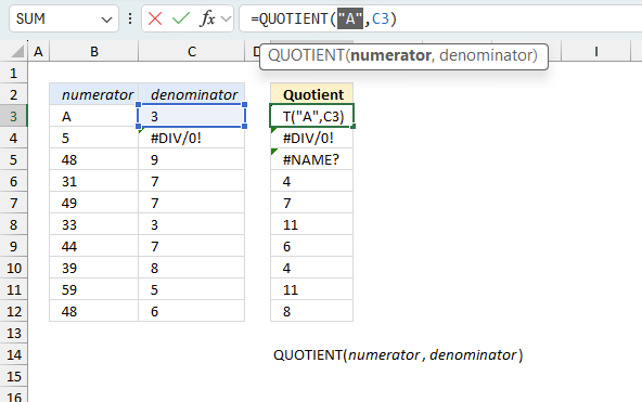
- Enter Edit mode: Double-press with left mouse button on the cell or press F2 to enter Edit mode for the formula.
- Select part of the formula: Highlight the specific part of the formula you want to evaluate. You can select and evaluate any part of the formula that could work as a standalone formula.
- Press F9: This will calculate and display the result of just that selected portion.
- Evaluate step-by-step: You can select and evaluate different parts of the formula to see intermediate results.
- Check for errors: This allows you to pinpoint which part of a complex formula may be causing an error.
The image above shows cell reference C3 converted to hard-coded value using the F9 key. The QUOTIENT function requires numerical values which is not the case in this example. We have found what is wrong with the formula.
Tips!
- View actual values: Selecting a cell reference and pressing F9 will show the actual values in those cells.
- Exit safely: Press Esc to exit Edit mode without changing the formula. Don't press Enter, as that would replace the formula part with the calculated value.
- Full recalculation: Pressing F9 outside of Edit mode will recalculate all formulas in the workbook.
Remember to be careful not to accidentally overwrite parts of your formula when using F9. Always exit with Esc rather than Enter to preserve the original formula. However, if you make a mistake overwriting the formula it is not the end of the world. You can “undo” the action by pressing keyboard shortcut keys CTRL + z or pressing the “Undo” button
7.3 Other errors
Floating-point arithmetic may give inaccurate results in Excel - Article
Floating-point errors are usually very small, often beyond the 15th decimal place, and in most cases don't affect calculations significantly.
Useful links
QUOTIENT function - Microsoft
QUOTIENT
'QUOTIENT' function examples
What is the MOD function? The Mod function returns the remainder after a number is divided by a divisor. The […]
The picture above shows data presented in only one column (column B), this happens sometimes when you get an undesired […]
Functions in 'Math and trigonometry' category
The QUOTIENT function function is one of 62 functions in the 'Math and trigonometry' category.
Excel function categories
Excel categories
3 Responses to “How to use the QUOTIENT function”
Leave a Reply
How to comment
How to add a formula to your comment
<code>Insert your formula here.</code>
Convert less than and larger than signs
Use html character entities instead of less than and larger than signs.
< becomes < and > becomes >
How to add VBA code to your comment
[vb 1="vbnet" language=","]
Put your VBA code here.
[/vb]
How to add a picture to your comment:
Upload picture to postimage.org or imgur
Paste image link to your comment.
With INT formula you will get same result. =INT(B2/C2)
Sorry, I did not read carefully...
you also mentioned this function.
[…] More MOD examples: Learn how the MOD function works, Quotient, Mod and Int functions […]