How to use the MAX function
What is the MAX function?
The MAX function calculates the largest number in a cell range or array.
Table of contents
- Introduction
- Syntax
- Arguments
- Function not working
- Get largest number based on a condition
- Get largest number based on multiple conditions
- For text
- Ignore #N/A error
- Second highest
- Second-highest number no duplicates
- Second-highest number based on a condition
- Get the highest number within each row
- Sort rows by their highest number within each row
- Get the highest number within each column
- Sort columns by their highest number within each row
1. Introduction
When is the MAX function useful in statistics?
The MAX function allows you to find the the maximum or highest value in a set of data points. This can be helpful when you want to identify outliers or extreme values in your dataset.
The range of a dataset is the difference between the maximum and minimum values. You can use the MAX function in combination with the MIN function to calculate the range which is a measure of the spread of the data.
2. Syntax
MAX(number1, [number2], ...)
3. Arguments
| Argument | Text |
| number1 | You need at least one argument. Required. |
| [number2] | Up to 254 arguments are possible. Optional. |
Arguments can be constants, named ranges, cell references, and arrays. The MAX function ignores text and boolean values, however not errors.
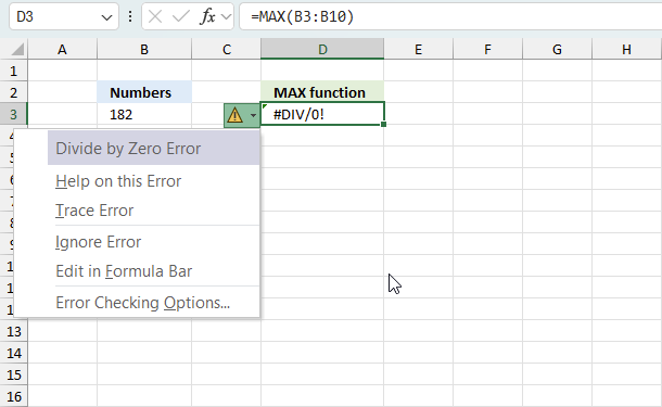
4. Function not working

A #NAME? error is most often the result of a misspelled function. The image above shows the MAX function in cell D3, however, it returns a #NAME? error. This example shows that the MAX function is misspelled and that the formula returns a #NAME! error.
4.1 Error in data

The MAX function can't handle error values in your data. The first error parsed is returned. The image above shows a #DIV/0! error in cell D3, data in cell B3:B10 contains a #DIV/0 error in cell B5.
Use the IFERROR function to catch and ignore error values in a specific range or array. It allows you to replace errors with any value, for example, a text value, numerical value or a boolean value. If we use the example demonstrated in the image above the formula becomes slightly larger and needs to be entered as an array formula if you use an Excel version earlier than Excel 365.
Formula in cell D3:
=MAX(IFERROR(B3:B10,""))
The formula above replaces errors with a blank value "", the MAX function then ignores the blank value and returns number 182. The downside with the IFERROR function is that it can be hard to spot errors because you will never be warned, everything looks fine when in fact you may need to fix the error.
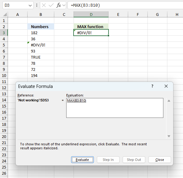
4.3 Troubleshooting the error value
When you encounter an error value in a cell a warning symbol appears, displayed in the image above. Press with mouse on it to see a pop-up menu that lets you get more information about the error.
- The first line describes the error if you press with left mouse button on it.
- The second line opens a pane that explains the error in greater detail.
- The third line takes you to the "Evaluate Formula" tool, a dialog box appears allowing you to examine the formula in greater detail.
- This line lets you ignore the error value meaning the warning icon disappears, however, the error is still in the cell.
- The fifth line lets you edit the formula in the Formula bar.
- The sixth line opens the Excel settings so you can adjust the Error Checking Options.
Here are a few of the most common Excel errors you may encounter.
#NULL error - This error occurs most often if you by mistake use a space character in a formula where it shouldn't be. Excel interprets a space character as an intersection operator. If the ranges don't intersect an #NULL error is returned. The #NULL! error occurs when a formula attempts to calculate the intersection of two ranges that do not actually intersect. This can happen when the wrong range operator is used in the formula, or when the intersection operator (represented by a space character) is used between two ranges that do not overlap. To fix this error double check that the ranges referenced in the formula that use the intersection operator actually have cells in common.
#SPILL error - The #SPILL! error occurs only in version Excel 365 and is caused by a dynamic array being to large, meaning there are cells below and/or to the right that are not empty. This prevents the dynamic array formula expanding into new empty cells.
#DIV/0 error - This error happens if you try to divide a number by 0 (zero) or a value that equates to zero which is not possible mathematically.
#VALUE error - The #VALUE error occurs when a formula has a value that is of the wrong data type. Such as text where a number is expected or when dates are evaluated as text.
#REF error - The #REF error happens when a cell reference is invalid. This can happen if a cell is deleted that is referenced by a formula.
#NAME error - The #NAME error happens if you misspelled a function or a named range.
#NUM error - The #NUM error shows up when you try to use invalid numeric values in formulas, like square root of a negative number.
#N/A error - The #N/A error happens when a value is not available for a formula or found in a given cell range, for example in the VLOOKUP or MATCH functions.
#GETTING_DATA error - The #GETTING_DATA error shows while external sources are loading, this can indicate a delay in fetching the data or that the external source is unavailable right now.
4.4 The formula returns an unexpected value
To understand why a formula returns an unexpected value we need to examine the calculations steps in detail. Luckily, Excel has a tool that is really handy in these situations. Here is how to troubleshoot a formula:
- Select the cell containing the formula you want to examine in detail.
- Go to tab “Formulas” on the ribbon.
- Press with left mouse button on "Evaluate Formula" button. A dialog box appears.
The formula appears in a white field inside the dialog box. Underlined expressions are calculations being processed in the next step. The italicized expression is the most recent result. The buttons at the bottom of the dialog box allows you to evaluate the formula in smaller calculations which you control. - Press with left mouse button on the "Evaluate" button located at the bottom of the dialog box to process the underlined expression.
- Repeat pressing the "Evaluate" button until you have seen all calculations step by step. This allows you to examine the formula in greater detail and hopefully find the culprit.
- Press "Close" button to dismiss the dialog box.

There is also another way to debug formulas using the function key F9. F9 is especially useful if you have a feeling that a specific part of the formula is the issue, this makes it faster than the "Evaluate Formula" tool since you don't need to go through all calculations to find the issue..
- Enter Edit mode: Double-press with left mouse button on the cell or press F2 to enter Edit mode for the formula.
- Select part of the formula: Highlight the specific part of the formula you want to evaluate. You can select and evaluate any part of the formula that could work as a standalone formula.
- Press F9: This will calculate and display the result of just that selected portion.
- Evaluate step-by-step: You can select and evaluate different parts of the formula to see intermediate results.
- Check for errors: This allows you to pinpoint which part of a complex formula may be causing an error.
The image above shows cell reference B3:B10 converted to hard-coded value using the F9 key. The MAX function requires non-error values which is not the case in this example. We have found what is wrong with the formula.
Tips!
- View actual values: Selecting a cell reference and pressing F9 will show the actual values in those cells.
- Exit safely: Press Esc to exit Edit mode without changing the formula. Don't press Enter, as that would replace the formula part with the calculated value.
- Full recalculation: Pressing F9 outside of Edit mode will recalculate all formulas in the workbook.
Remember to be careful not to accidentally overwrite parts of your formula when using F9. Always exit with Esc rather than Enter to preserve the original formula. However, if you make a mistake overwriting the formula it is not the end of the world. You can “undo” the action by pressing keyboard shortcut keys CTRL + z or pressing the “Undo” button
4.5 Other errors
Floating-point arithmetic may give inaccurate results in Excel - Article
Floating-point errors are usually very small, often beyond the 15th decimal place, and in most cases don't affect calculations significantly.
5. Based on a condition

This example demonstrates how to find the maximum number based on a specific condition given in cell F2. The image above shows a data table in cell range B2:C10, here is the data:
| Color | Number |
| Blue | 10 |
| Yellow | 50 |
| Yellow | 40 |
| Blue | 10 |
| Yellow | 20 |
| Blue | 40 |
| Blue | 10 |
| Yellow | 20 |
The condition is "Blue" and the formula takes only the corresponding values on the same row in C3:C10 into the calculation.
Array formula in cell F3:
The condition "Blue" is found in cells B3, B6, B8, and B9. The corresponding numbers in C3:C10 are 10, 10, 40, and 10. The largest number is 40 which is also displayed in cell F3.
5.1 Explaining formula in cell F3
The Evaluate Formula tool is located on the Formulas tab in the Ribbon. It is a useful feature that allows you to step through and evaluate complex formulas to understand how the calculation is being performed and identify any errors or issues. The following steps shows these detailed evaluations for the formula above.
Step 1 - Compare values
The equal sign lets you compare value to value, the result is a boolean value TRUE or FALSE.
F2=B3:B10
becomes
"Blue"={"Blue"; "Yellow"; "Yellow"; "Blue"; "Yellow"; "Blue"; "Blue"; "Yellow"}
and returns
{TRUE; FALSE; FALSE; TRUE; FALSE; TRUE; TRUE; FALSE}.
Step 2 - Evaluate IF function
The IF function returns one value if the logical test is TRUE and another value if the logical test is FALSE.
IF(logical_test, [value_if_true], [value_if_false])
IF(F2=B3:B10, C3:C10, "")
becomes
IF({TRUE; FALSE; FALSE; TRUE; FALSE; TRUE; TRUE; FALSE}, C3:C10, "")
becomes
IF({TRUE; FALSE; FALSE; TRUE; FALSE; TRUE; TRUE; FALSE}, {10; 50; 40; 10; 20; 40; 10; 20}, "")
and returns
{10; ""; ""; 10; ""; 40; 10; ""}.
Step 3 - Return max number
The MAX function calculates the largest number in a cell range.
MAX(number1, [number2], ...)
MAX(IF(F2=B3:B10, C3:C10, ""))
becomes
MAX({10; ""; ""; 10; ""; 40; 10; ""})
and returns 40 in cell F3.
6. Get the largest number based on multiple conditions

The image above shows a formula in cell G3 that extracts the largest number if the adjacent value is equal to the criteria specified in cell E3:E4.
The conditions in cells E3:E4 are "Blue" and "Yellow" respectively. The data table in B2:C10 is:
| Color | Number |
| Blue | 10 |
| Yellow | 50 |
| Green | 40 |
| Blue | 10 |
| Yellow | 20 |
| Green | 40 |
| Blue | 10 |
| Green | 20 |
"Blue" or "Yellow" are found in cells B3, B4, B6, B7, and B9. The corresponding numbers in C3:C10 are 10, 50, 10, 20, and 10.
Array formula in cell G3:
The largest number in the data set is 50 which is also displayed in cell G3.
6.1 Explaining formula in cell F3
The Evaluate Formula tool is located on the Formulas tab in the Ribbon. It is a useful feature that allows you to step through and evaluate complex formulas to understand how the calculation is being performed and identify any errors or issues. The following steps shows these detailed evaluations for the formula above.
Step 1 - Identify cells equal to any of the criteria
The COUNTIF function calculates the number of cells equal to a condition.
COUNTIF(range, criteria)
COUNTIF(E3:E4,B3:B10)
becomes
COUNTIF({"Blue"; "Yellow"},{"Blue"; "Yellow"; "Green"; "Blue"; "Yellow"; "Green"; "Blue"; "Green"})
and returns {1; 1; 0; 1; 1; 0; 1; 0}. 1 means that the value in that position is equal to one of the conditions, this means that the position in the array is important in order to extract correct numbers.
Step 2 - Replace 1 with the corresponding number
The IF function returns one value if the logical test is TRUE and another value if the logical test is FALSE.
IF(logical_test, [value_if_true], [value_if_false])
IF(COUNTIF(E3:E4, B3:B10), C3:C10, "")
becomes
IF({1; 1; 0; 1; 1; 0; 1; 0}, C3:C10, "")
becomes
IF({1; 1; 0; 1; 1; 0; 1; 0}, {10; 50; 40; 10; 20; 40; 10; 20}, "")
and returns {10; 50; ""; 10; 20; ""; 10; ""}.
Step 3 - Return the largest number in the array
The MAX function calculates the largest number in a cell range.
MAX(number1, [number2], ...)
MAX(IF(COUNTIF(E3:E4, B3:B10), C3:C10, ""))
becomes
MAX({10; 50; ""; 10; 20; ""; 10; ""})
and returns 50 in cell G3.
7. Find the text string with the largest number of characters

The following section explains how to filter the largest value based on the number of characters in a cell. If you are looking for the most repeated value go to section 6.2 below.
Cell range B2:B12 contains the following values:
| Text |
| Emphasis |
| Basil |
| Boolean |
| Emphasis |
| Gift |
| Historian |
| Boolean |
| Pension |
| Emphasis |
| Yogurt |
The character count is:
| 8 | Emphasis |
| 5 | Basil |
| 7 | Boolean |
| 5 | Death |
| 4 | Gift |
| 9 | Historian |
| 11 | Integration |
| 7 | Pension |
| 7 | Poverty |
| 6 | Yogurt |
The formula counts the number of characters of each cell value and the MAX function calculates the largest number. The formula then gets the largest value based on character count and returns the result in cell D3.
Array formula in cell D3:
Value "Integration" is the largest value based on the number of characters in cell range B3:B12.
7.1 Explaining formula in cell F3
The Evaluate Formula tool is located on the Formulas tab in the Ribbon. It is a useful feature that allows you to step through and evaluate complex formulas to understand how the calculation is being performed and identify any errors or issues. The following steps shows these detailed evaluations for the formula above.
Step 1 - Count characters
The LEN function counts the number of characters in a cell.
LEN(B3:B12)
becomes
LEN({"Emphasis"; "Basil"; "Boolean"; "Doors"; "Gift"; "Historian"; "Integration"; "Pension"; "Poverty"; "Yogurt"})
and returns {8; 5; 7; 5; 4; 9; 11; 7; 7; 6}.
Step 2 - Get largest character count
The MAX function calculates the largest number in a cell range.
MAX(number1, [number2], ...)
MAX(LEN(B3:B12))
becomes
MAX({8; 5; 7; 5; 4; 9; 11; 7; 7; 6})
and returns 11.
Step 3 - Find the position of a cell containing the largest number of characters
The MATCH function returns the relative position of an item in an array or cell reference that matches a specified value in a specific order.
MATCH(lookup_value, lookup_array, [match_type])
MATCH(MAX(LEN(B3:B12)), LEN(B3:B12), 0)
becomes
MATCH(11, {8; 5; 7; 5; 4; 9; 11; 7; 7; 6}, 0)
and returns 7.
Step 4 - Get value based on position
The INDEX function returns a value from a cell range, you specify which value based on a row and column number.
INDEX(B3:B12, MATCH(MAX(LEN(B3:B12)), LEN(B3:B12), 0))
becomes
INDEX(B3:B12, 7)
becomes
INDEX({"Emphasis"; "Basil"; "Boolean"; "Death"; "Gift"; "Historian"; "Integration"; "Pension"; "Poverty"; "Yogurt"}, 7)
and returns "Integration" in cell D3.
7.2 Get the most frequent value

The formula below extracts the most repeated text value in cell range B3:B12. The values are:
| Text |
| Emphasis |
| Basil |
| Boolean |
| Emphasis |
| Gift |
| Historian |
| Boolean |
| Pension |
| Emphasis |
| Yogurt |
The frequency or count is:
| 3 | Emphasis |
| 1 | Basil |
| 2 | Boolean |
| 3 | Emphasis |
| 1 | Gift |
| 1 | Historian |
| 2 | Boolean |
| 1 | Pension |
| 3 | Emphasis |
| 1 | Yogurt |
The table above shows the frequency of each value, "Emphasis" exists three times in cell range B3:B12.
Formula in cell D3:
"Emphasis" is the most frequent value in B3:B12, the formula returns this value in cell D3. However, use the MODE function if you are working with numbers. This single function is easier to work with than the formula I created above.
7.2.1 Explaining formula in cell D3
The Evaluate Formula tool is located on the Formulas tab in the Ribbon. It is a useful feature that allows you to step through and evaluate complex formulas to understand how the calculation is being performed and identify any errors or issues. The following steps shows these detailed evaluations for the formula above.
Step 1 - Count value frequency
The COUNTIF function calculates the number of cells equal to a condition.
COUNTIF(range, criteria)
COUNTIF(B3:B12, B3:B12)
becomes
COUNTIF({"Emphasis"; "Basil"; "Boolean"; "Emphasis"; "Gift"; "Historian"; "Boolean"; "Pension"; "Emphasis"; "Yogurt"},{"Emphasis"; "Basil"; "Boolean"; "Emphasis"; "Gift"; "Historian"; "Boolean"; "Pension"; "Emphasis"; "Yogurt"})
and returns
{3; 1; 2; 3; 1; 1; 2; 1; 3; 1}.

The array is displayed in cell range A3:A12, each number corresponds on the same row to a value in B3:B12. Cell value in B3 is found three times in B3:B12, the array shows 3 in cell A3.
Step 2 - Get most frequent value
The MAX function calculates the largest number in a cell range.
MAX(number1, [number2], ...)
MAX(COUNTIF(B3:B12, B3:B12))
becomes
MAX({3; 1; 2; 3; 1; 1; 2; 1; 3; 1})
and returns 3.
Step 3 - Find position of most frequent value
The MATCH function returns the relative position of an item in an array or cell reference that matches a specified value in a specific order.
MATCH(lookup_value, lookup_array, [match_type])
MATCH(MAX(COUNTIF(B3:B12, B3:B12)), COUNTIF(B3:B12, B3:B12), 0)
becomes
MATCH(3, COUNTIF(B3:B12, B3:B12), 0)
becomes
MATCH(3, {3; 1; 2; 3; 1; 1; 2; 1; 3; 1}, 0)
and returns 1.
Step 4 - Get most frequent value
The INDEX function returns a value from a cell range, you specify which value based on a row and column number (optional).
INDEX(reference, row, column)
INDEX(B3:B12, MATCH(MAX(COUNTIF(B3:B12, B3:B12)), COUNTIF(B3:B12, B3:B12), 0))
becomes
INDEX(B3:B12, 1)
becomes
INDEX({"Emphasis"; "Basil"; "Boolean"; "Emphasis"; "Gift"; "Historian"; "Boolean"; "Pension"; "Emphasis"; "Yogurt"}, 1)
and returns "Emphasis".
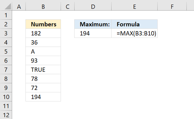
8. Ignore #N/A error

This formula returns the largest number from a given cell range ignoring possible #N/A errors. The data table, shown in cell range B2:B10 in the image above, is:
| Numbers |
| 182 |
| 36 |
| #N/A |
| 93 |
| TRUE |
| 78 |
| 72 |
| 194 |
Cell B5 contains a #N/A error which usually breaks the MAX function, however, the formula below converts #N/A errors to a blank value "".
Array formula in cell D3:
The formula ignores the #N/A error and returns 194 which is the largest number in cell range B3:B10.
8.1 Explaining formula
The Evaluate Formula tool is located on the Formulas tab in the Ribbon. It is a useful feature that allows you to step through and evaluate complex formulas to understand how the calculation is being performed and identify any errors or issues. The following steps shows these detailed evaluations for the formula above.
Step 1 - Identify #N/A errors
The ISNA function returns TRUE if a value is a #N/A error.
ISNA(value)
ISNA(B3:B10)
becomes
ISNA({182; 36; #N/A; 93; TRUE; 78; 72; 194})
and returns
{FALSE; FALSE; TRUE; FALSE; FALSE; FALSE; FALSE; FALSE}.
Step 2 - Replace #N/A errors with a blank
The IF function returns one value if the logical test is TRUE and another value if the logical test is FALSE.
IF(logical_test, [value_if_true], [value_if_false])
IF(ISNA(B3:B10), "", B3:B10)
becomes
IF({FALSE; FALSE; TRUE; FALSE; FALSE; FALSE; FALSE; FALSE}, "", {182; 36; #N/A; 93; TRUE; 78; 72; 194})
and returns
{182; 36; ""; 93; TRUE; 78; 72; 194}.
The N/A error is replaced with a blank in the array above.
Step 3 - Extract the largest number ignoring blanks and text values
MAX(IF(ISNA(B3:B10), "", B3:B10))
becomes
MAX({182; 36; ""; 93; TRUE; 78; 72; 194})
and returns 194.
9. Second-highest number

The image above demonstrates a formula in cell E2 that extracts the second largest number from cell range B3:B10. The values are:
| Number |
| 10 |
| 50 |
| 40 |
| 10 |
| 20 |
| 30 |
| 10 |
| 20 |
Formula in cell E2:
The LARGE function extracts the k-th largest number in a cell range or array. In this example, k is 2 meaning the second largest.
LARGE(array, k)
10. Second-highest number no duplicates

The image above demonstrates a formula in cell E2 that extracts the second largest number, duplicate numbers are ignored. The data table is:
| Number |
| 10 |
| 50 |
| 40 |
| 10 |
| 20 |
| 30 |
| 10 |
| 20 |
For example, both cells B4 and B8 contain the number 50. The LARGE function returns the second largest number considering duplicate numbers as well. The following function ignores duplicates returning 40 in cell E4.
Array formula in cell E2:
10.1 Explaining formula in cell E2
The Evaluate Formula tool is located on the Formulas tab in the Ribbon. It is a useful feature that allows you to step through and evaluate complex formulas to understand how the calculation is being performed and identify any errors or issues. The following steps shows these detailed evaluations for the formula above.
Step 1 - Find the largest number
The MAX function calculates the largest number in a cell range.
MAX(number1, [number2], ...)
MAX(B3:B10)
becomes
MAX({10; 50; 40; 10; 20; 50; 10; 20})
and returns 50.
Step 2 - Find the largest number
The equal sign lets you compare value to value, the result is a boolean value TRUE or FALSE.
MAX(B3:B10)=B3:B10
becomes
50={10; 50; 40; 10; 20; 50; 10; 20}
and returns
{FALSE; TRUE; FALSE; FALSE; FALSE; TRUE; FALSE; FALSE}.
Step 3 - Replace boolean value TRUE with corresponding numbers
The IF function returns one value if the logical test is TRUE and another value if the logical test is FALSE.
IF(logical_test, [value_if_true], [value_if_false])
IF(MAX(B3:B10)=B3:B10, "", B3:B10)
becomes
IF({FALSE; TRUE; FALSE; FALSE; FALSE; TRUE; FALSE; FALSE}, "", B3:B10)
becomes
IF({FALSE; TRUE; FALSE; FALSE; FALSE; TRUE; FALSE; FALSE}, "", {10; 50; 40; 10; 20; 50; 10; 20})
and returns
{""; 50; ""; ""; ""; 50; ""; ""}.
Step 4 - Extract maximum number from array
MAX(IF(MAX(B3:B10)=B3:B10, "", B3:B10))
becomes
MAX({""; 50; ""; ""; ""; 50; ""; ""})
and returns 50.
11. Second-highest number based on a condition

This example demonstrates a formula that extracts the second largest number based on a condition applied to an adjacent column. The data table is:
| Color | Number |
| Blue | 10 |
| Yellow | 50 |
| Yellow | 40 |
| Blue | 10 |
| Yellow | 20 |
| Blue | 50 |
| Blue | 10 |
| Yellow | 20 |
The conditions is specified in cell F2 and is "Blue", the matching cells in cell range B3:B10 are B3, B6, B8, and B9.
Formula in cell F3:
The corresponding cell values are 10, 10, 50, and 10. The second largest value is 10.
11.1 Explaining formula
The Evaluate Formula tool is located on the Formulas tab in the Ribbon. It is a useful feature that allows you to step through and evaluate complex formulas to understand how the calculation is being performed and identify any errors or issues. The following steps shows these detailed evaluations for the formula above.
Step 1 - Identify values equal to condition
The equal sign lets you compare value to value, in this case, value to array. The result is a boolean value TRUE or FALSE.
F2=B3:B10
becomes
"Blue"={"Blue"; "Yellow"; "Yellow"; "Blue"; "Yellow"; "Blue"; "Blue"; "Yellow"}
and returns
{TRUE; FALSE; FALSE; TRUE; FALSE; TRUE; TRUE; FALSE}.
Step 2 - Replace TRUE with corresponding number on the same row
The IF function returns one value if the logical test is TRUE and another value if the logical test is FALSE.
IF(logical_test, [value_if_true], [value_if_false])
IF(F2=B3:B10, C3:C10, "")
becomes
IF({TRUE; FALSE; FALSE; TRUE; FALSE; TRUE; TRUE; FALSE}, {10; 50; 40; 10; 20; 50; 10; 20}, "")
and returns
{10; ""; ""; 10; ""; 50; 10; ""}.
Step 3 - Extract second largest number from the array
The LARGE function extracts the k-th largest number in a cell range or array.
LARGE(array, k)
LARGE(IF(F2=B3:B10, C3:C10, ""), 2)
becomes
LARGE({10; ""; ""; 10; ""; 50; 10; ""}, 2)
and returns 10.
12. Get the highest number within each row

The image above shows an Excel 365 dynamic array formula that calculates the max number for each row in cell range B3:E9. The data table is:
| 66 | 36 | 68 | 28 |
| 63 | 67 | 97 | 16 |
| 31 | 79 | 43 | 12 |
| 89 | 1 | 32 | 41 |
| 55 | 11 | 27 | 78 |
| 42 | 36 | 87 | 56 |
| 42 | 44 | 98 | 37 |
The first row is 66, 36, 68, and 28. The largest value is 68 which is displayed in cell G3.
Excel 365 formula in cell G3:
The formula in cell G3 calculates the maximum number for each row meaning the result is an array of values. In other words, the formula spills values to cells below as far as needed. This formula works only in Excel 365.
Why calculate the maximum values per row for the entire range in one single formula? This allows us to do more complicated calculations like sorting the rows based on their largest numbers. This was not possible in earlier Excel versions, you had to rely on autofilter, Excel tables or other tools. Section 13 describes how to sort the rows based on their corresponding maximum numbers.
Explaining formula
The Evaluate Formula tool is located on the Formulas tab in the Ribbon. It is a useful feature that allows you to step through and evaluate complex formulas to understand how the calculation is being performed and identify any errors or issues. The following steps shows these detailed evaluations for the formula above.
Step 1 - Count cells only numbers
The MAX function calculate the largest number in a cell range.
Function syntax: MAX(number1, [number2], ...)
MAX(a)
Step 2 - Build the LAMBDA function
The LAMBDA function build custom functions without VBA, macros or javascript.
Function syntax: LAMBDA([parameter1, parameter2, …,] calculation)
LAMBDA(a,MAX(a))
Step 3 - Count nonempty cells per row
The BYROW function puts values from an array into a LAMBDA function row-wise.
Function syntax: BYROW(array, lambda(array, calculation))
BYROW(B3:E9,LAMBDA(a,MAX(a)))
13. Sort rows by their highest number within each row

This example demonstrates an Excel 365 formula that calculates the largest number per row and then sorts the rows, from large to small, based on their largest numbers. The data table contains these numbers:
| 66 | 36 | 68 | 28 |
| 63 | 67 | 97 | 16 |
| 31 | 79 | 43 | 12 |
| 89 | 1 | 32 | 41 |
| 55 | 11 | 27 | 78 |
| 42 | 36 | 87 | 56 |
| 42 | 44 | 98 | 37 |
The largest number per row is the following array: {68;97;79;89;78;87;98}
Excel 365 dynamic array formula in cell G3:
The data table after being sorted becomes this:
| 42 | 44 | 98 | 37 |
| 63 | 67 | 97 | 16 |
| 89 | 1 | 32 | 41 |
| 42 | 36 | 87 | 56 |
| 31 | 79 | 43 | 12 |
| 55 | 11 | 27 | 78 |
| 66 | 36 | 68 | 28 |
This is what the formula in cell G3 returns, it spills values to cells below and to the right as far as needed. The first row contains number 98, this number is the largest in the entire table, this is why this row is placed on top.
The next row has number 97 as the largest number, this number is the second largest number in the entire data table. That is why it is located in row 2.
Explaining formula
This formula works just like the example in section 12, but it also sorts rows based on the max number in each row. Column K shows the largest number found in each row in cell range G3:J9.
The SORTBY function sorts a cell range or array based on values in a corresponding range or array.
Function syntax: SORTBY(array, by_array1, [sort_order1], [by_array2, sort_order2],…)
14. Get the highest number within each column

The image above shows an Excel 365 dynamic array formula that returns an array containing the maximum number per column for cell range B3:E9. This is the data table:
| 66 | 36 | 68 | 28 |
| 63 | 67 | 97 | 16 |
| 31 | 79 | 43 | 12 |
| 89 | 1 | 32 | 41 |
| 55 | 11 | 27 | 78 |
| 42 | 36 | 87 | 56 |
| 42 | 44 | 98 | 37 |
Excel 365 formula in cell B11:
The formula returns the following array: {89,79,98,78} It is spilled to cell B11 and cells to the right horizontally. This array tells us that the largest number in the first column is 89, the second column is 79, the third column is 98 and the last column has 78 as the highest number.
Explaining formula
The Evaluate Formula tool is located on the Formulas tab in the Ribbon. It is a useful feature that allows you to step through and evaluate complex formulas to understand how the calculation is being performed and identify any errors or issues. The following steps shows these detailed evaluations for the formula above.
Step 1 - Count numbers
The MAX function calculate the largest number in a cell range.
Function syntax: MAX(number1, [number2], ...)
MAX(a)
Step 2 - Build the LAMBDA function
The LAMBDA function build custom functions without VBA, macros or javascript.
Function syntax: LAMBDA([parameter1, parameter2, …,] calculation)
LAMBDA(a,MAX(a))
Step 3 - Count numbers per column
The BYCOL function passes all values in a column based on an array to a LAMBDA function, the LAMBDA function calculates new values based on a formula you specify.
Function syntax: BYCOL(array, lambda(array, calculation))
BYCOL(B3:E9,LAMBDA(a,MAX(a)))
15. Sort columns by their highest number within each column

This example demonstrates an Excel 365 formula that calculates the largest number per column and then sorts the columns, from large to small, based on their largest numbers. The data table contains these numbers:
| 66 | 36 | 68 | 28 |
| 63 | 67 | 97 | 16 |
| 31 | 79 | 43 | 12 |
| 89 | 1 | 32 | 41 |
| 55 | 11 | 27 | 78 |
| 42 | 36 | 87 | 56 |
| 42 | 44 | 98 | 37 |
The largest number per column is the following array: {89,79,98,78}
Excel 365 dynamic array formula in cell G3:
The data table after being sorted becomes this:
| 68 | 66 | 36 | 28 |
| 97 | 63 | 67 | 16 |
| 43 | 31 | 79 | 12 |
| 32 | 89 | 1 | 41 |
| 27 | 55 | 11 | 78 |
| 87 | 42 | 36 | 56 |
| 98 | 42 | 44 | 37 |
This is what the formula in cell G3 returns, it spills values to cells below and to the right as far as needed. The first column contains number 98, this number is the largest in the entire table, this is why this column is first counting from left to right.
The next column has number 89 as the largest number which is the second largest considering values per column.
The third column has number 79 as the largest number which is the third largest. The fourth and last column has number 78 as the largest number which is the fourth largest.
15.1 Explaining formula
This formula works just like the example in section 14, however, it also sorts the columns based on the largest number found in each column.
The SORTBY function sorts a cell range or array based on values in a corresponding range or array.
Function syntax: SORTBY(array, by_array1, [sort_order1], [by_array2, sort_order2],…)
'MAX' function examples
Table of Contents How to use the BETADIST function How to use the BETAINV function How to use the BINOMDIST […]
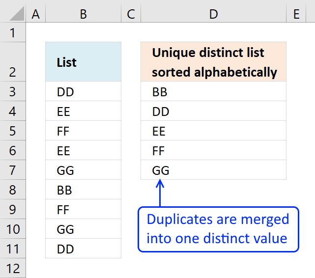
This article demonstrates Excel formulas that allows you to list unique distinct values from a single column and sort them […]
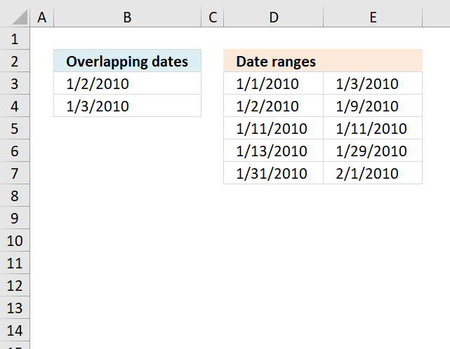
The array formula in cell B3 extracts overlapping dates based on the date ranges in columns D and E. What's […]
Functions in 'Statistical' category
The MAX function function is one of 73 functions in the 'Statistical' category.
How to comment
How to add a formula to your comment
<code>Insert your formula here.</code>
Convert less than and larger than signs
Use html character entities instead of less than and larger than signs.
< becomes < and > becomes >
How to add VBA code to your comment
[vb 1="vbnet" language=","]
Put your VBA code here.
[/vb]
How to add a picture to your comment:
Upload picture to postimage.org or imgur
Paste image link to your comment.
Contact Oscar
You can contact me through this contact form