How to use the DATEVALUE function

What is the DATEVALUE function?
The DATEVALUE function returns an Excel date value (serial number) based on a date stored as text.
Table of Contents
1. Introduction
What are dates in Excel?
Dates are stored numerically but formatted to display in human-readable date/time formats, this enables Excel to do work with dates in calculations.

For example, dates are stored as sequential serial numbers with 1 being January 1, 1900 by default. The integer part (whole number) represents the date the decimal part represents the time.
This allows dates to easily be formatted to display in many date/time formats like mm/dd/yyyy, dd/mm/yyyy and so on and still be part of calculations as long as the date is stored numerically in a cell.
You can try this yourself, type 10000 in a cell, press CTRL + 1 and change the cell's formatting to date, press with left mouse button on OK. The cell now shows 5/18/1927.
Why are dates stored as text in Excel?
Dates are not stored as text in Excel they are stored as numbers, however, Excel tries to identify values as text, numbers, Boolean values, dates, and time automatically but may fail in rare occasions.
This may happen when you import data from the internet, databases, text files, and other sources. You can convert the dates to Excel dates if you like but it can be a tedious and time consuming task.
The DATEVALUE function lets you convert the text date in the formula to an Excel date without you first converting them on the worksheet.
How to enter valid dates in Excel?

Valid dates are right-aligned in a cell just like numbers, invalid dates are identified as text values and left-aligned. The image above shows that / (forward slash) and - (dash) are valid delimiting characters in Excel dates, demonstrated in cells B2 and B3.
A dot and no delimiters at all, shown in cells B4 and B5, are invalid, these dates are left-aligned by Excel. The DATEVALUE cant properly identify these date values either, you need to change these dates by hand or using the methods described below.
2. Syntax
DATEVALUE(date_text)
3. Arguments
| date_text | Required. The date stored as text you want to convert to an Excel date (serial number). |
4. Example
A date stored as text can't be sorted, filtered or be used in Excel date calculations. You need to convert the date stored as text to a date that Excel recognizes. The image above shows dates stored as text in cell range B3:B7.
Formula in cell C3:
Explaining formula
DATEVALUE(B3)
becomes
DATEVALUE("1/4/2013")
and returns
41278 which is the corresponding serial number Excel uses for the date "1/4/2013".
5. Function not working
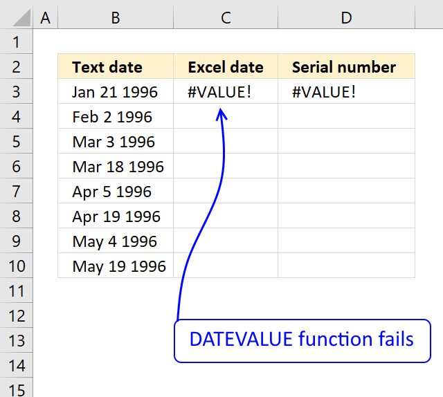
The DATEVALUE function returns an Excel date value (serial number) based on a date stored as text. However, it must be a valid text date which is determined by your date and time settings (national settings) on your operating system.
Formula in cell C3:
5.1. Verify your date and time settings

Microsoft recommends that you verify your date and time settings so they are compatible with the text date format. On a "Windows 10" operating system open the Control Panel and then "National Settings" and see if you can find a supported date setting. Both the short and long dates must match.
5.2. Convert a text date to an Excel date using a formula
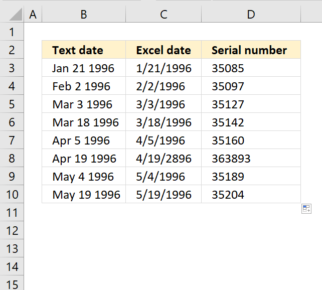
I could not find a setting that worked with the text date above so I created the following formula in cell C3.
The picture above shows the output of the formula in column C.
5.2.3. Explaining the formula in cell C3
Step 1 - Extract year from string
To extract the year from the text date in cell B3 I simply use the RIGHT function to extract the 4 last characters.
The RIGHT function extracts a specific number of characters always starting from the right.
RIGHT(text,[num_chars])
RIGHT(B3, 4)
becomes
RIGHT("Jan 21 1996", 4)
and returns 1996.
Step 2 - Extract month abbreviation from string
The month number is a little harder since it is built of three letters. To get the three letters from B3 I use the LEFT function.
The LEFT function extracts a specific number of characters always starting from the left.
LEFT(text, [num_chars])
LEFT(B3, 3)
becomes
LEFT("Jan 21 1996", 3)
and returns "Jan".
Step 3 - Convert month to a number
The MATCH function returns the relative position of an item in an array or cell reference that matches a specified value in a specific order.
MATCH(lookup_value, lookup_array, [match_type])
MATCH(LEFT(B3, 3), {"Jan"; "Feb"; "Mar"; "Apr"; "May"; "Jun"; "Jul"; "Aug"; "Sep"; "Oct"; "Nov"; "Dec"}, 0)
becomes
MATCH("Jan", {"Jan"; "Feb"; "Mar"; "Apr"; "May"; "Jun"; "Jul"; "Aug"; "Sep"; "Oct"; "Nov"; "Dec"}, 0)
and returns 1. "Jan" is the first value in the array.
Step 4 - Extract day from string
The MID function returns a substring from a string based on the starting position and the number of characters you want to extract.
MID(text, start_num, num_chars)
MID(B3, 4, 3)
becomes
MID("Jan 21 1996", 4, 3)
and returns " 21".
Step 5 - Create an Excel date
The DATE function allows you to create an Excel date based on a year, month, and day number.
The arguments are DATE(year, month, day).
DATE(RIGHT(B3, 4), MATCH(LEFT(B3, 3), {"Jan"; "Feb"; "Mar"; "Apr"; "May"; "Jun"; "Jul"; "Aug"; "Sep"; "Oct"; "Nov"; "Dec"}, 0), MID(B3, 4, 3))
becomes
DATE(1996, 1, 21)
and returns 1/21/1996 in cell C3.
Get Excel *.xlsx file
DATEVALUE function not working.xlsx
5.3 Example

This example shows that the DATEVALUE function can't handle a date with a dot as a delimiting character.
Formula in cell D3:
The DATEVALUE function returns a #VALUE! error.
How to create an Excel date from dates using dots as delimiting characters?
The SUBSTITUTE function lets you replace a given text string with a new text string.
Formula in cell D3 that works:
Explaining formula
Step 1 - Substitute dots with forward slash
The SUBSTITUTE function replaces a specific text string in a value. Case sensitive.
Function syntax: SUBSTITUTE(text, old_text, new_text, [instance_num])
SUBSTITUTE(B3,".","/")
becomes
SUBSTITUTE("1.4.2013",".","/")
and returns
"1/4/2013".
Step 2 - Convert text date to an Excel date
The DATEVALUE function returns an Excel date value (serial number) based on a date stored as text.
Function syntax: DATEVALUE(date_text)
DATEVALUE(SUBSTITUTE(B3,".","/"))
becomes
DATEVALUE("1/4/2013")
and returns 41278. Here is how to format the cell value as a date:
- Select the cell (D3).
- Press CTRL + 1 to open the "Format Cells.." dialog box.

- Select category : Date
- Pick a date formatting.
- Press with mouse on the "OK" button.

This example shows that the DATEVALUE function can't handle a date without delimiting characters.
Formula in cell D3:
The DATEVALUE function returns a #VALUE! error.
How to create an Excel date from dates without delimiting characters?
Formula in cell D3 that works:
Explaining formula
Step 1 - Extract year from date
The RIGHT function extracts a specific number of characters always starting from the right.
Function syntax: RIGHT(text,[num_chars])
RIGHT(B3,4)
becomes
RIGHT("01042013",4)
and returns "2013".
Step 2 - Extract month from date
The LEFT function extracts a specific number of characters always starting from the left.
Function syntax: LEFT(text, [num_chars])
LEFT(B3,2)
becomes
LEFT("01042013",2)
and returns "01".
Step 3 - Extract day from date
The MID function returns a substring from a string based on the starting position and the number of characters you want to extract.
Function syntax: MID(text, start_num, num_chars)
MID(B3,3,2)
becomes
MID("01042013",3,2)
and returns "04".
Step 4 - Convert to an Excel date
The DATE function returns a number that acts as a date in the Excel environment.
Function syntax: DATE(year, month, day)
DATE(RIGHT(B3,4),LEFT(B3,2),MID(B3,3,2))
becomes
DATE("2013","01","04")
and returns 41278.
5.4 Errors
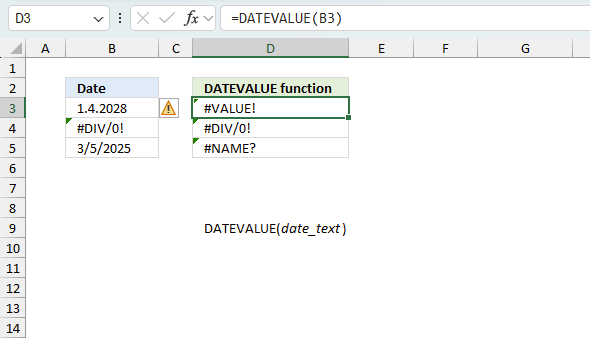
The DATEVALUE function returns
- #VALUE! error if you use an invalid date value.
- #NAME? error if you misspell the function name.
- propagates errors, meaning that if the input contains an error (e.g., #VALUE!, #REF!), the function will return the same error.
5.5 Troubleshooting the error value
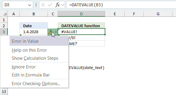
When you encounter an error value in a cell a warning symbol appears, displayed in the image above. Press with mouse on it to see a pop-up menu that lets you get more information about the error.
- The first line describes the error if you press with left mouse button on it.
- The second line opens a pane that explains the error in greater detail.
- The third line takes you to the "Evaluate Formula" tool, a dialog box appears allowing you to examine the formula in greater detail.
- This line lets you ignore the error value meaning the warning icon disappears, however, the error is still in the cell.
- The fifth line lets you edit the formula in the Formula bar.
- The sixth line opens the Excel settings so you can adjust the Error Checking Options.
Here are a few of the most common Excel errors you may encounter.
#NULL error - This error occurs most often if you by mistake use a space character in a formula where it shouldn't be. Excel interprets a space character as an intersection operator. If the ranges don't intersect an #NULL error is returned. The #NULL! error occurs when a formula attempts to calculate the intersection of two ranges that do not actually intersect. This can happen when the wrong range operator is used in the formula, or when the intersection operator (represented by a space character) is used between two ranges that do not overlap. To fix this error double check that the ranges referenced in the formula that use the intersection operator actually have cells in common.
#SPILL error - The #SPILL! error occurs only in version Excel 365 and is caused by a dynamic array being to large, meaning there are cells below and/or to the right that are not empty. This prevents the dynamic array formula expanding into new empty cells.
#DIV/0 error - This error happens if you try to divide a number by 0 (zero) or a value that equates to zero which is not possible mathematically.
#VALUE error - The #VALUE error occurs when a formula has a value that is of the wrong data type. Such as text where a number is expected or when dates are evaluated as text.
#REF error - The #REF error happens when a cell reference is invalid. This can happen if a cell is deleted that is referenced by a formula.
#NAME error - The #NAME error happens if you misspelled a function or a named range.
#NUM error - The #NUM error shows up when you try to use invalid numeric values in formulas, like square root of a negative number.
#N/A error - The #N/A error happens when a value is not available for a formula or found in a given cell range, for example in the VLOOKUP or MATCH functions.
#GETTING_DATA error - The #GETTING_DATA error shows while external sources are loading, this can indicate a delay in fetching the data or that the external source is unavailable right now.
5.6 The formula returns an unexpected value
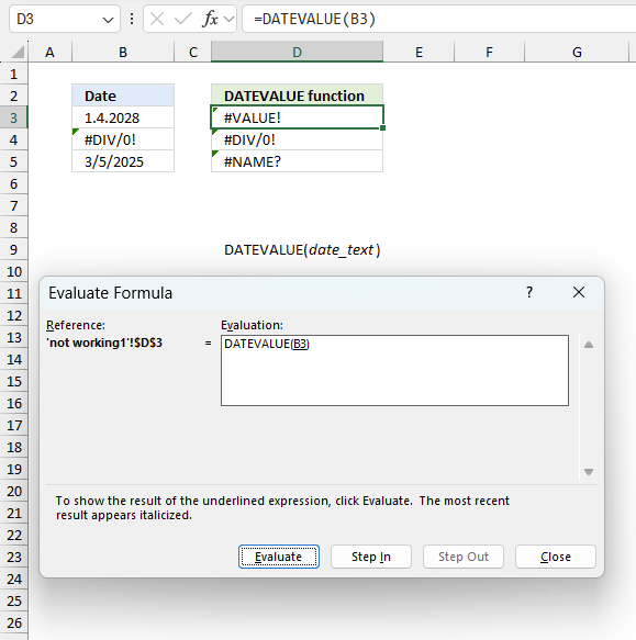
To understand why a formula returns an unexpected value we need to examine the calculations steps in detail. Luckily, Excel has a tool that is really handy in these situations. Here is how to troubleshoot a formula:
- Select the cell containing the formula you want to examine in detail.
- Go to tab “Formulas” on the ribbon.
- Press with left mouse button on "Evaluate Formula" button. A dialog box appears.
The formula appears in a white field inside the dialog box. Underlined expressions are calculations being processed in the next step. The italicized expression is the most recent result. The buttons at the bottom of the dialog box allows you to evaluate the formula in smaller calculations which you control. - Press with left mouse button on the "Evaluate" button located at the bottom of the dialog box to process the underlined expression.
- Repeat pressing the "Evaluate" button until you have seen all calculations step by step. This allows you to examine the formula in greater detail and hopefully find the culprit.
- Press "Close" button to dismiss the dialog box.
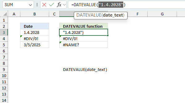
There is also another way to debug formulas using the function key F9. F9 is especially useful if you have a feeling that a specific part of the formula is the issue, this makes it faster than the "Evaluate Formula" tool since you don't need to go through all calculations to find the issue..
- Enter Edit mode: Double-press with left mouse button on the cell or press F2 to enter Edit mode for the formula.
- Select part of the formula: Highlight the specific part of the formula you want to evaluate. You can select and evaluate any part of the formula that could work as a standalone formula.
- Press F9: This will calculate and display the result of just that selected portion.
- Evaluate step-by-step: You can select and evaluate different parts of the formula to see intermediate results.
- Check for errors: This allows you to pinpoint which part of a complex formula may be causing an error.
The image above shows cell reference B3 converted to hard-coded value using the F9 key. The DATEVALUE function requires valid Excel dates which is not the case in this example. We have found what is wrong with the formula.
Tips!
- View actual values: Selecting a cell reference and pressing F9 will show the actual values in those cells.
- Exit safely: Press Esc to exit Edit mode without changing the formula. Don't press Enter, as that would replace the formula part with the calculated value.
- Full recalculation: Pressing F9 outside of Edit mode will recalculate all formulas in the workbook.
Remember to be careful not to accidentally overwrite parts of your formula when using F9. Always exit with Esc rather than Enter to preserve the original formula. However, if you make a mistake overwriting the formula it is not the end of the world. You can “undo” the action by pressing keyboard shortcut keys CTRL + z or pressing the “Undo” button
5.7 Other errors
Floating-point arithmetic may give inaccurate results in Excel - Article
Floating-point errors are usually very small, often beyond the 15th decimal place, and in most cases don't affect calculations significantly.
'DATEVALUE' function examples
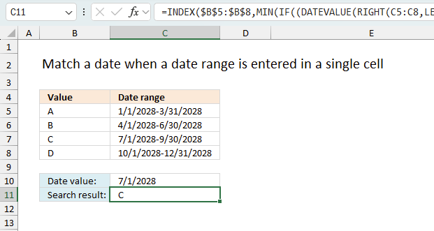
This article explains how to search for a specific date and identify a date range in which it falls between […]
Functions in 'Date and Time' category
The DATEVALUE function function is one of 22 functions in the 'Date and Time' category.
Excel function categories
Excel categories
2 Responses to “How to use the DATEVALUE function”
Leave a Reply
How to comment
How to add a formula to your comment
<code>Insert your formula here.</code>
Convert less than and larger than signs
Use html character entities instead of less than and larger than signs.
< becomes < and > becomes >
How to add VBA code to your comment
[vb 1="vbnet" language=","]
Put your VBA code here.
[/vb]
How to add a picture to your comment:
Upload picture to postimage.org or imgur
Paste image link to your comment.
Hi, Oscar
Result 4/19/2896 is strange.
Alternative formula...
=--SUBSTITUTE(TRIM(B3)," ",", ",2)
aMareis,
Result 4/19/2896 is strange.
I didn't see that. Yes, there is a space character that makes it weird.
=--SUBSTITUTE(TRIM(B3)," ",", ",2)
Great formula, thanks for your valuable comment.