How to use the LEFT function
What is the LEFT function?
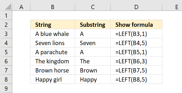
The LEFT function extracts a specific number of characters always starting from the left. It is one of the most used functions for text manipulation.
What is the difference between the LEFT function and the LEFTB function?
The LEFT and LEFTB functions handle character counting differently based on your default language setting in Excel. LEFTB is designed for double-byte languages like Chinese, Japanese, Korean. It counts each double-byte character as 2 when a DBCS language is set as the default.
LEFT always counts each character as 1, single-byte or double-byte, regardless of language setting. So LEFTB will count each double byte character as 2 contrary to the LEFT for the same text in a DBCS language.
Japanese, Chinese (Simplified), Chinese (Traditional), and Korean are some examples of languages supporting DBCS.
Table of Contents
1. Syntax
The LEFT function has two arguments, the second argument is optional. It defaults to 1 meaning the first character from the left is extracted if the second argument is omitted.
LEFT(text, [num_chars])
2. Arguments
| text | Text string or a cell reference to a text string. |
| [num_chars] | The number of characters to extract. Optional. If this argument is not entered only the first character is extracted. |
3. Example

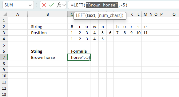
The formula in cell D7 demonstrated in the image above extracts the first five letters from the value in cell B7.
Formula in cell D7:
The image above shows the string "Brown horse", each cell is numbered from 1 to 11.
The formula =LEFT(B7, 5) extracts the five first characters from the left which is "Brown".
4. Until character

The image above demonstrates a formula in cell D3 that extracts characters from left until a specified character is found. In this case / (forward slash).
Formula in cell D3:
This formula in Excel calculates the leftmost part of a text string in cell B3, up to the position where the text in cell C3 is found. For example, if B3 contains “11/1/2022” and C3 contains "/", then the function will return "11".
Explaining formula
Step 1 - Search string for given character
The SEARCH function returns a number representing the position of character at which a specific text string is found reading left to right.
SEARCH(find_text,within_text, [start_num])
SEARCH(C3, B3)
becomes
SEARCH("/","11/1/2022")
and returns 3.
Step 2 - Subtract with 1
The minus character lets you subtract numbers in an Excel formula.
SEARCH(C3, B3)-1
becomes
3-1 equals 2.
Step 3 - Extract given number of characters from left
LEFT(B3, SEARCH(C3, B3)-1)
becomes
LEFT(B3, 2)
becomes
LEFT("11/1/2022", 2)
and returns "11".
5. Until space

Formula in cell C3:
This formula returns the leftmost part of a text string in cell B3, up to the position where the first space character is found. For example, if B3 contains “Green tomatoes”, then the function will return “Green”.
Explaining formula
Step 1 - Find space character in string
The SEARCH function returns a number representing the position of character at which a specific text string is found reading left to right.
SEARCH(find_text,within_text, [start_num])
SEARCH(" ", B3)
becomes
SEARCH(" ","Green tomatoes")
and returns 6. The space character is the sixth character in the string.
Step 2 - Subtract number with 1
The minus character lets you subtract numbers in an Excel formula.
SEARCH(" ", B3)-1
becomes
6-1 equals 5.
Step 3 - Extract a given number of characters from left
LEFT(B3, SEARCH(" ", B3)-1)
becomes
LEFT(B3, 5)
becomes
LEFT("Green tomatoes", 5)
and returns "Green".
6. Extract characters until second space is found

The picture above shows a formula in cell C3 that extracts a string from cell B3 until the second space character from the left.
Formula in cell C3:
This formula above returns the leftmost part of a text string in cell B3, up to the position where the second space character is replaced by a vertical bar. For example, if B3 contains “Green delicious tomatoes”, then the function will return “Green delicious”.
Explaining formula
Step 1 - Replace second space character
The SUBSTITUTE function allows you to replace a given string of characters, it also lets you choose which instance. I am using a character not being used in the string in this case |
SUBSTITUTE(text, old_text, new_text, [instance_num])
SUBSTITUTE(B3," ","|",2)
becomes
SUBSTITUTE("Green delicious tomatoes"," ","|",2)
and returns "Green delicious|tomatoes". The second space character is now |.
Step 2 - Find position of character
The SEARCH function returns a number representing the position of character at which a specific text string is found reading left to right.
SEARCH(find_text,within_text, [start_num])
SEARCH("|", SUBSTITUTE(B3," ","|",2))
becomes
SEARCH("|", "Green delicious|tomatoes")
and returns 16.
Step 3 - Extract a given number of characters from left
LEFT(B3,SEARCH("|", SUBSTITUTE(B3," ","|",2)))
becomes
LEFT(B3, 16)
becomes
LEFT("Green delicious tomatoes", 16)
and returns "Green delicious".
7. Extract characters until a dash

The following formula extracts characters until a dash character.
Formula in cell C3:
For example, if cell B3 contains "Green-tomatoes" then the formula returns "Green.
Explaining formula
Step 1 - Find the position of dash character
The SEARCH function returns a number representing the position of character at which a specific text string is found reading left to right.
SEARCH(find_text,within_text, [start_num])
SEARCH("-", B3)
becomes
SEARCH("-", "Green-tomatoes")
and returns 6.
Step 2 - Subtract with 1
The minus character lets you subtract numbers in an Excel formula.
SEARCH("-", B3)-1
becomes
6-1 equals 5.
Step 3 - Extract a given number of characters from left
LEFT(B3, SEARCH("-", B3)-1)
becomes
LEFT(B3, 5)
becomes
LEFT("Green-tomatoes", 5)
and returns "Green".
8. Extract characters until a number

Array formula in cell C3:
This calculates the leftmost part of a text string in cell B3 up to the position where the first number is found. For example, if B3 contains “Green4tomatoes”, then the function will return “Green”. The function uses an array formula to search for each digit from 0 to 9 in the text and returns the smallest position where a digit is found.
8.1 How to enter an array formula

Excel 365 users can ignore these instructions, enter the formula as a regular formula.
- Copy array formula.
- Double press on cell C3, a prompt appears.
- Paste array formula to the cell.
- Press and hold CTRL + SHIFT keys simultaneously.
- Press Enter once.
- Release all keys.
A beginning and ending curly bracket is now shown, don't enter these characters yourself. They appear automatically, see the image above.
8.2 Explaining array formula
Step 1 - Search for numbers between 0 (zero) and 9
The SEARCH function returns a number representing the position of character at which a specific text string is found reading left to right.
SEARCH(find_text,within_text, [start_num])
returns {#VALUE!; ... ; #VALUE!}.
The SEARCH function returns #VALUE! error if nothing found.
Step 2 - Subtract with 1
The minus character lets you subtract numbers in an Excel formula.
SEARCH({0; 1; 2; 3; 4; 5; 6; 7; 8; 9}, B3)-1
returns {#VALUE!; ... ; #VALUE!}
Step 3 - Handle errors
The IFERROR function lets you catch most errors in Excel formulas, it returns TRUE if value is an error and FALSE if not.
IFERROR(value, value_if_error)
IFERROR(SEARCH({0; 1; 2; 3; 4; 5; 6; 7; 8; 9}, B3)-1, "")
returns {""; ""; ""; ""; 5; ""; ""; ""; ""; ""}.
Step 4 - Extrcat smallest number
The MIN function returns the minimum number in a cell range or array, it ignores text and blank values.
MIN(number1, [number2], ...)
MIN(IFERROR(SEARCH({0; 1; 2; 3; 4; 5; 6; 7; 8; 9}, B3)-1, ""))
becomes
MIN({""; ""; ""; ""; 5; ""; ""; ""; ""; ""})
and returns 5.
Step 5 -
LEFT(B3, MIN(IFERROR(SEARCH({0; 1; 2; 3; 4; 5; 6; 7; 8; 9}, B3)-1, "")))
9. Remove characters from left until a space character is found

The image above shows a formula in cell C3 that removes the first characters from the left until a space character is found. A space character is found in the second position, the first and second character is removed.
Formula in cell C3:
The formula uses the SEARCH function to find the position of the first space character in the text and then replaces all the characters from the first position to that position with nothing. For example, if B3 contains “A ABCD-123”, then the function will return “ABCD-123”.
Explaining formula
Step 1 - Find first space character
The SEARCH function returns a number representing the position of character at which a specific text string is found reading left to right.
SEARCH(find_text,within_text, [start_num])
SEARCH(" ",B3)
becomes
SEARCH(" ","A ABCD-123")
and returns 2.
Step 2 - Replace characters with nothing
The REPLACE function replaces part of a text string, based on the character position, and the number of characters, with a different text string.
REPLACE(old_text, start_num, num_chars, new_text)
REPLACE(B3,1,SEARCH(" ",B3),"")
becomes
REPLACE(B3,1,2,"")
becomes
REPLACE("A ABCD-123", 1, 2,"")
and returns "ABCD-123".
10. Extract first three numbers from the left

The formula in cell C3 extracts the three first numbers in cell B3, note that there are other characters than numbers between the numbers as well.
Array formula in cell C3:
10.1 Explaining formula
Step 1 - Count characters
The LEN function calculates the number of characters in a value.
LEN(value)
LEN(B3)
becomes
LEN("A 2BV3 5C523Ds")
and returns 14.
Step 2 - Create a cell range containing as many rows as there are characters in cell B3
The INDEX function returns a value based on a row and column number, however, it can also build a cell reference.
A1:INDEX(A:A,LEN(B3))
becomes
A1:INDEX(A:A,14)
and returns A1:A14.
Step 3 - Create an array of row numbers
The ROW function returns a number representing the row based on a cell reference. It also returns an array of row numbers if a cell reference containing multiple rows is used.
ROW(A1:INDEX(A:A,LEN(B3)))
becomes
ROW(A1:A14)
and returns {1; 2; ... ; 14}.
Step 4 - Split value in cell B3 to an array containing a character each
The MID function returns a substring from a string based on the starting position and the number of characters you want to extract.
MID(text, start_num, num_chars)
MID(B3,ROW(A1:INDEX(A:A,LEN(B3))),1)
returns {"A"; " "; "2"; "B"; "V"; "3"; " "; "5"; "C"; "5"; "2"; "3"; "D"; "s"}.
Step 5 - Add 0 (zero) to each character
Adding zero to each value allws us to identify if a value is a number or not.
MID(B3,ROW(A1:INDEX(A:A,LEN(B3))),1)+0
returns {#VALUE!; #VALUE!; 2; ... ; #VALUE!}.
Step 6 - Replace error values with blanks
The IFERROR function handles errors in an Excel formula.
IFERROR(value, value_if_error)
IFERROR(MID(B3,ROW(A1:INDEX(A:A,LEN(B3))),1)+0,"")
returns {""; ""; 2; ""; ""; 3; ""; 5; ""; 5; 2; 3; ""; ""}.
Note that the error values are replaced with a blank "".
Step 7 - Join numbers
The TEXTJOIN function concatenates text strings.
TEXTJOIN(delimiter, ignore_empty, text1, [text2], ...)
TEXTJOIN("",TRUE,IFERROR(MID(B3,ROW(A1:INDEX(A:A,LEN(B3))),1)+0,""))
becomes
TEXTJOIN("", TRUE, {""; ""; 2; ""; ""; 3; ""; 5; ""; 5; 2; 3; ""; ""})
and returns "235523".
Step 8 - Extract first three numbers from string
LEFT(TEXTJOIN("",TRUE,IFERROR(MID(B3,ROW(A1:INDEX(A:A,LEN(B3))),1)+0,"")),3)
becomes
LEFT("235523",3)
and returns "235".
12. Function not working
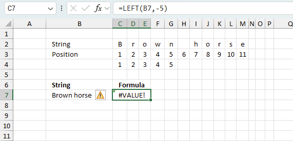
The LEFT function returns
- #VALUE! error if you use a negative number or a text value in the [num_chars] argument.
- #NAME? error if you misspell the function name.
- propagates errors, meaning that if the input contains an error (e.g., #VALUE!, #REF!), the function will return the same error.
12.1 Troubleshooting the error value
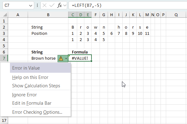
When you encounter an error value in a cell a warning symbol appears, displayed in the image above. Press with mouse on it to see a pop-up menu that lets you get more information about the error.
- The first line describes the error if you press with left mouse button on it.
- The second line opens a pane that explains the error in greater detail.
- The third line takes you to the "Evaluate Formula" tool, a dialog box appears allowing you to examine the formula in greater detail.
- This line lets you ignore the error value meaning the warning icon disappears, however, the error is still in the cell.
- The fifth line lets you edit the formula in the Formula bar.
- The sixth line opens the Excel settings so you can adjust the Error Checking Options.
Here are a few of the most common Excel errors you may encounter.
#NULL error - This error occurs most often if you by mistake use a space character in a formula where it shouldn't be. Excel interprets a space character as an intersection operator. If the ranges don't intersect an #NULL error is returned. The #NULL! error occurs when a formula attempts to calculate the intersection of two ranges that do not actually intersect. This can happen when the wrong range operator is used in the formula, or when the intersection operator (represented by a space character) is used between two ranges that do not overlap. To fix this error double check that the ranges referenced in the formula that use the intersection operator actually have cells in common.
#SPILL error - The #SPILL! error occurs only in version Excel 365 and is caused by a dynamic array being to large, meaning there are cells below and/or to the right that are not empty. This prevents the dynamic array formula expanding into new empty cells.
#DIV/0 error - This error happens if you try to divide a number by 0 (zero) or a value that equates to zero which is not possible mathematically.
#VALUE error - The #VALUE error occurs when a formula has a value that is of the wrong data type. Such as text where a number is expected or when dates are evaluated as text.
#REF error - The #REF error happens when a cell reference is invalid. This can happen if a cell is deleted that is referenced by a formula.
#NAME error - The #NAME error happens if you misspelled a function or a named range.
#NUM error - The #NUM error shows up when you try to use invalid numeric values in formulas, like square root of a negative number.
#N/A error - The #N/A error happens when a value is not available for a formula or found in a given cell range, for example in the VLOOKUP or MATCH functions.
#GETTING_DATA error - The #GETTING_DATA error shows while external sources are loading, this can indicate a delay in fetching the data or that the external source is unavailable right now.
12.2 The formula returns an unexpected value
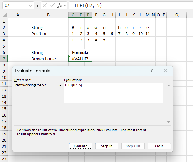
To understand why a formula returns an unexpected value we need to examine the calculations steps in detail. Luckily, Excel has a tool that is really handy in these situations. Here is how to troubleshoot a formula:
- Select the cell containing the formula you want to examine in detail.
- Go to tab “Formulas” on the ribbon.
- Press with left mouse button on "Evaluate Formula" button. A dialog box appears.
The formula appears in a white field inside the dialog box. Underlined expressions are calculations being processed in the next step. The italicized expression is the most recent result. The buttons at the bottom of the dialog box allows you to evaluate the formula in smaller calculations which you control. - Press with left mouse button on the "Evaluate" button located at the bottom of the dialog box to process the underlined expression.
- Repeat pressing the "Evaluate" button until you have seen all calculations step by step. This allows you to examine the formula in greater detail and hopefully find the culprit.
- Press "Close" button to dismiss the dialog box.
There is also another way to debug formulas using the function key F9. F9 is especially useful if you have a feeling that a specific part of the formula is the issue, this makes it faster than the "Evaluate Formula" tool since you don't need to go through all calculations to find the issue..
- Enter Edit mode: Double-press with left mouse button on the cell or press F2 to enter Edit mode for the formula.
- Select part of the formula: Highlight the specific part of the formula you want to evaluate. You can select and evaluate any part of the formula that could work as a standalone formula.
- Press F9: This will calculate and display the result of just that selected portion.
- Evaluate step-by-step: You can select and evaluate different parts of the formula to see intermediate results.
- Check for errors: This allows you to pinpoint which part of a complex formula may be causing an error.
The image above shows cell reference B7 converted to hard-coded value using the F9 key, however there is nothing wrong with the first argument.The second argument is -5. the LEFT function requires positive numerical values which is not the case in this example. We have found what is wrong with the formula.
Tips!
- View actual values: Selecting a cell reference and pressing F9 will show the actual values in those cells.
- Exit safely: Press Esc to exit Edit mode without changing the formula. Don't press Enter, as that would replace the formula part with the calculated value.
- Full recalculation: Pressing F9 outside of Edit mode will recalculate all formulas in the workbook.
Remember to be careful not to accidentally overwrite parts of your formula when using F9. Always exit with Esc rather than Enter to preserve the original formula. However, if you make a mistake overwriting the formula it is not the end of the world. You can “undo” the action by pressing keyboard shortcut keys CTRL + z or pressing the “Undo” button
12.3 Other errors
Floating-point arithmetic may give inaccurate results in Excel - Article
Floating-point errors are usually very small, often beyond the 15th decimal place, and in most cases don't affect calculations significantly.
Useful resources
LEFT function - Microsoft
Excel LEFT function with formula examples
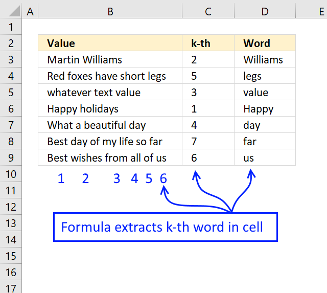
'LEFT' function examples

This post explains how to lookup a value and return multiple values. No array formula required.
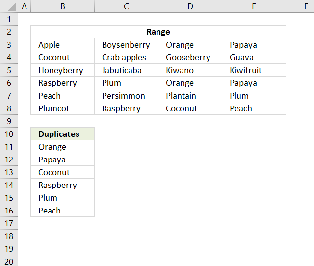
This article describes two formulas that extract duplicates from a multi-column cell range, the first one is built for Excel […]
Whether you're cleaning up imported data, parsing product names, or building dynamic spreadsheets, mastering text manipulation in Excel can save […]
Functions in 'Text' category
The LEFT function function is one of 29 functions in the 'Text' category.
Excel function categories
Excel categories
2 Responses to “How to use the LEFT function”
Leave a Reply
How to comment
How to add a formula to your comment
<code>Insert your formula here.</code>
Convert less than and larger than signs
Use html character entities instead of less than and larger than signs.
< becomes < and > becomes >
How to add VBA code to your comment
[vb 1="vbnet" language=","]
Put your VBA code here.
[/vb]
How to add a picture to your comment:
Upload picture to postimage.org or imgur
Paste image link to your comment.
this didn't work. multiplying by one only creates a #value! error.
Jeffery
The first three characters are numbers?