Extract unique distinct values from an Excel Table filtered list

This article demonstrates two formulas that extract distinct values from a filtered Excel Table, one formula for Excel 365 subscribers and the other formula for earlier Excel versions.
Table of Contents
- List unique distinct values in a filtered Excel defined Table - Excel 365
- List unique distinct values - Autofilter
- List unique distinct values in a filtered Excel defined Table - earlier Excel versions
- List unique distinct values in a filtered Excel defined Table - User Defined Function
- Get Excel *.xlsx file
- Filter duplicate records - Autofilter
- Count unique distinct values in a filtered Excel defined Table
- Populate drop down list with filtered Excel Table values
1. Extract unique distinct values in a filtered Excel defined Table - Excel 365
Excel 365 dynamic array formula in cell B26:
Dynamic array formulas and spilled array behavior
Explaining the formula in cell B26
Step 1 - Count rows
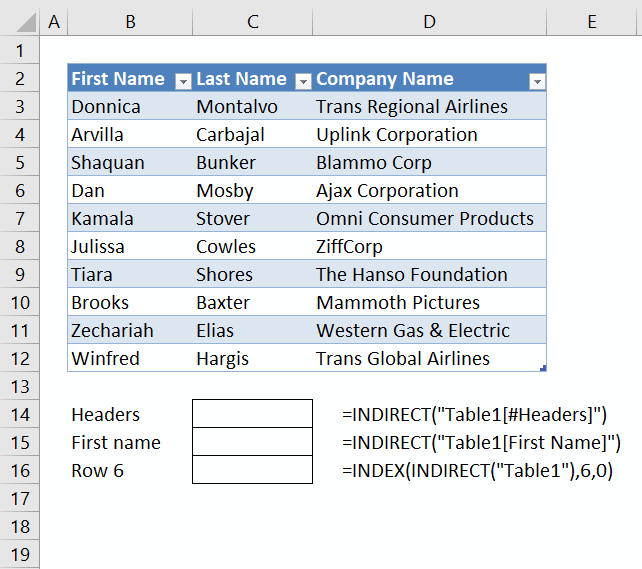
Table2[First Name] is a structured reference meaning a cell reference to an Excel Table. This particular name references a column with column header name "First Name" in Excel Table Table2.
The ROWS function calculate the number of rows in a cell range.
Function syntax: ROWS(array)
ROWS(Table2[First Name])
returns 20.
Step 2 - Create a sequence from 1 to n
The SEQUENCE function creates a list of sequential numbers.
Function syntax: SEQUENCE(rows, [columns], [start], [step])
SEQUENCE(ROWS(Table2[First Name]))
returns {1; 2; ... ; 20}.
Step 3 - Create a sequence from 0 (zero) to n-1
The minus sign lets you subtract numbers in an Excel formula, this works fine with arrays as well.
SEQUENCE(ROWS(Table2[First Name]))-1
returns {0; 1; ... ; 19}.
Step 4 - Create an array that works with the SUBTOTAL function
The OFFSET function returns a reference to a range that is a given number of rows and columns from a given reference.
Function syntax: OFFSET(reference,rows,columns,[height],[width])
OFFSET(Table2[First Name], SEQUENCE(ROWS(Table2[First Name]))-1, 0, 1)
returns
{"Kaya"; "Fraser"; ...; "Kaya"}.
Step 5 - Check which values are displayed
The SUBTOTAL function returns a subtotal from a list or database, you can choose from a variety of arguments that determine what you want the function to do.
Function syntax: SUBTOTAL(function_num, ref1, ...)
SUBTOTAL(3, OFFSET(Table2[First Name], SEQUENCE(ROWS(Table2[First Name]))-1, 0, 1))
returns {1; 1; ... ; 1}.
Step 6 - Filter values based on count
The FILTER function extracts values/rows based on a condition or criteria.
Function syntax: FILTER(array, include, [if_empty])
FILTER(Table2[First Name], SUBTOTAL(3, OFFSET(Table2[First Name], SEQUENCE(ROWS(Table2[First Name]))-1, 0, 1)))
returns {"Kaya"; "Fraser"; ... ; "Kaya"}.
Step 7 - Extract unique distinct values
The UNIQUE function returns a unique or unique distinct list.
Function syntax: UNIQUE(array,[by_col],[exactly_once])
UNIQUE(FILTER(Table2[First Name], SUBTOTAL(3, OFFSET(Table2[First Name], SEQUENCE(ROWS(Table2[First Name]))-1, 0, 1)))
returns {"Kaya"; "Fraser"; "Jui"; "Horace"; "Kelton"}.
Step 8 - Shorten the formula
The LET function lets you name intermediate calculation results which can shorten formulas considerably and improve performance.
Function syntax: LET(name1, name_value1, calculation_or_name2, [name_value2, calculation_or_name3...])
UNIQUE(FILTER(Table2[First Name], SUBTOTAL(3, OFFSET(Table2[First Name], SEQUENCE(ROWS(Table2[First Name]))-1, 0, 1)))
x - Table2[First Name]
LET(x, Table2[First Name], UNIQUE(FILTER(x, SUBTOTAL(3, OFFSET(x, SEQUENCE(ROWS(x))-1, 0, 1))))
2. Extract unique distinct values using a formula - Autofilter

The formulas work for Excel's Autofilter feature as well. The formula for earlier Excel versions is the same as in section three below but the structured references are now cell references. Read section three for a formula explanation.
Array formula in cell B26:
The formula for Excel 365 is the same as in section one above but the structured reference is now a cell reference. Read section one for a formula explanation.
Excel 365 dynamic array formula in cell D26:
Recommended reading
3. Extract unique distinct values from a filtered Excel defined Table - earlier Excel versions
Oscar,
I am using the VBA code & FilterUniqueSort array to generate unique lists that drive Selection Change AutoFilter on multiple colums. Is there a way to make the list only return the unique values that are visible in the filtered source data?
I see a similar answer above using just an array formula, but my source is too long for that to be practical. Any help would be greatly appreciated.
Robert Jr
Array formula
I modified a formula by Laurent Longre found here: Excel Experts E-letter from John Walkenbach's web site.
Array Formula in cell B26:
To enter an array formula, type the formula in a cell then press and hold CTRL + SHIFT simultaneously, now press Enter once. Release all keys.
The formula bar now shows the formula with a beginning and ending curly bracket telling you that you entered the formula successfully. Don't enter the curly brackets yourself.
3.1 Explaining array formula in cell B26
Step 1 - Create an array
This step is necessary in order to be able to use the SUBTOTAL function in the next step. The ROW function returns row numbers based on a cell reference.
The MATCH function converts the row number array to an array that starts with 1.
OFFSET(Table2[First Name], MATCH(ROW(Table2[First Name]), ROW(Table2[First Name]))-1, 0, 1)
becomes
OFFSET({"Kaya"; "Fraser"; ... ; "Kaya"}, {0; 1; ... ; 19}, 0, 1)
The OFFSET function creates an array of arrays that the SUBTOTAL function can process.
returns { {"Kaya"}; {"Fraser"}; ... ; {"Kaya"} }
Step 2 - Which values are hidden?
The SUBTOTAL function will in this step count each array in the array as one and return 1 if the value is nonempty and is not visible. The first argument is 3 representing COUNTA function. It counts the number of cells that are not empty.
SUBTOTAL(3, OFFSET(Table2[First Name], MATCH(ROW(Table2[First Name]), ROW(Table2[First Name]))-1, 0, 1))
returns {1; 1; ... ; 1}.
This array tells us that the three first values in Table2[First Name] are visible, however, the fourth value is hidden etc. 1 - visible, 0 (zero) - hidden.
Step 3 - Convert 1 to 0 (zero)
The IF function has three arguments, the first one must be a logical expression. If the expression evaluates to TRUE then one thing happens (argument 2) and if FALSE another thing happens (argument 3).
IF(SUBTOTAL(3, OFFSET(Table2[First Name], MATCH(ROW(Table2[First Name]), ROW(Table2[First Name]))-1, 0, 1)), COUNTIF($B$25:B25, Table2[First Name]), "")
The COUNTIF function in this step will make sure that only unique distinct values are being returned, it contains an expanding cell reference that keeps track of previously displayed values.
IF(SUBTOTAL(3, OFFSET(Table2[First Name], MATCH(ROW(Table2[First Name]), ROW(Table2[First Name]))-1, 0, 1)), COUNTIF($B$25:B25, Table2[First Name]), "")
returns {0; 0; ... ; ""; 0; 0}
Step 4 - Find position
The MATCH function returns a number representing the position of the first 0 (zero) in the array.
MATCH(0, IF(SUBTOTAL(3, OFFSET(Table2[First Name], MATCH(ROW(Table2[First Name]), ROW(Table2[First Name]))-1, 0, 1)), COUNTIF($C$25:C25, Table2[First Name]),""), 0)
becomes
MATCH(0, {0; 0; ... ; ""; 0; 0}, 0) and returns 1.
Step 5 - Return value
The INDEX function returns a value based on cell reference and a row and column number.
INDEX(Table2[First Name], MATCH(0, IF(SUBTOTAL(3, OFFSET(Table2[First Name], MATCH(ROW(Table2[First Name]), ROW(Table2[First Name]))-1, 0, 1)), COUNTIF($C$25:C25, Table2[First Name]),""), 0))
becomes
INDEX(Table2[First Name], 1)
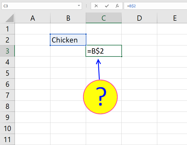
and returns "Kaya" in cell B26.
4. Extract unique distinct values from a filtered Excel defined Table - User defined Function
User defined function in cell range A26:A31:
This formula is also entered as an array formula.
4.1 User defined Function Syntax
FilterUniqueSortTable(rng)
4.2 Arguments
| Parameter | Text |
| rng | Required. A cell reference to the range in the Excel defined Table you want to extract unique distinct values from. |
4.3 VBA Code
'Name custom function and parameters
Function FilterUniqueSortTable(rng As Range)

'Declare variables and data types
Dim ucoll As New Collection, Value As Variant, temp() As Variant
Dim iRows As Single, i As Single

'Redimension array variable temp in order to be able to expand the variable later on
ReDim temp(0)

'Enable error handling
On Error Resume Next

'Iterate thorugh each value in cell range
For Each Value In rng

    'Check if cell is not empty and visible
    If Len(Value) > 0 And Value.EntireRow.Hidden = False Then

        'Add value to collection, this line will return an error if the value already exists in the collection
        ucoll.Add Value, CStr(Value)
    End If

'Continue with next value
Next Value

'Disable error handling
On Error GoTo 0

'Iterate through each value in collection
For Each Value In ucoll

    'Save value to array variable temp
    temp(UBound(temp)) = Value

    'Add another container to array variable temp
    ReDim Preserve temp(UBound(temp) + 1)

'Continue with next value
Next Value

'Remove last item from array variable temp
ReDim Preserve temp(UBound(temp) - 1)

'Count the number of rows the UDF is entered in by the user and save to variable iRows
iRows = Range(Application.Caller.Address).Rows.Count

'Use UDF SelectionSort to sort values from A to Z
SelectionSort temp

'Add items so the array variable temp has the same number of rows as the entered UDF and save blank values to items that contain nothing
For i = UBound(temp) To iRows
  ReDim Preserve temp(UBound(temp) + 1)
  temp(UBound(temp)) = ""
Next i

'Rearrange values in array variable temp and return them to worksheet
FilterUniqueSortTable = Application.Transpose(temp)
End Function
4.4 Where to copy code?

Press Alt+F11 to open VB Editor.
- Double press with left mouse button on your workbook in the Project Explorer.
- Press with left mouse button on "Insert" on the menu and then press with left mouse button on "Module".
- Paste above code to code module.
- Exit VB Editor and return to Excel.
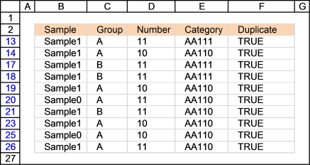
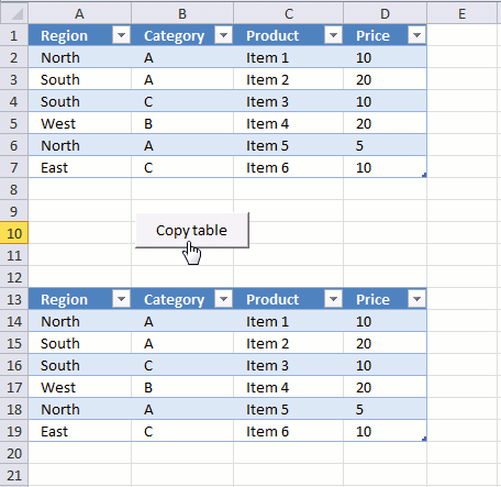
6. Filter duplicate records - Autofilter
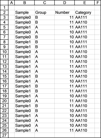
In this article I will demonstrate a technique to filter duplicate records. The picture below shows you a data set in columns B to E. Next step is to create an Excel defined table.
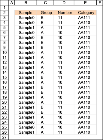
Press with left mouse button on a cell in the table, go to tab "Insert" on the ribbon. Press with left mouse button on "Insert Table" button. The following dialog box appears.
Press with left mouse button on OK button.
Type Duplicate in cell F2 and then use the following formula in cell F3:
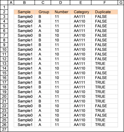
How the formula works in cell F13
Step 1 - Understand how relative and absolute cell references work
The formula uses absolute and relative cell references. In cell G3 the formula is:
=COUNTIFS($B$3:B3, B3, $C$3:C3, C3, $D$3:D3, D3, $E$3:E3, E3)>1
In cell G13 the formula has changed to:
=COUNTIFS($B$3:B13, B13, $C$3:C13, C13, $D$3:D13, D13, $E$3:E13, E13)>1
The cell ranges expand as the formula is copied to cells below. This lets you count the current record in above records.
Recommended articles
What is a reference in Excel? Excel has an A1 reference style meaning columns are named letters A to XFD […]
Step 2 - Find duplicates
COUNTIFS($B$3:B13, B13, $C$3:C13, C13, $D$3:D13, D13, $E$3:E13, E13)>1
becomes
=2>1
and returns TRUE in cell G13
Recommended articles
Checks multiple conditions against the same number of cell ranges and counts how many times all criteria are met.
Filter records based on formula
- Press with mouse on black arrow on cell F2
- Enable only value TRUE
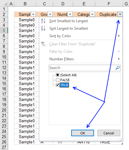
- Press with left mouse button on OK button
7. Count unique distinct values in a filtered Excel defined Table

This article demonstrates a formula that counts unique distinct values filtered from an Excel defined Table.
Debra Dalgleish described in an article how to create a Line Between Dates in Filtered List. She modified a formula by Laurent Longre found here: Excel Experts E-letter from John Walkenbach's web site.
I remember a post I did about extracting unique distinct values from a filtered table (udf and array formula that also was inspired by Laurent Longre's formula.
The Excel defined Table shown in the image above is named Table2. There are forenames in column A. The table is filtered with "Finland" and "Mexico" in column C, the following array formula counts unique distinct values based on a filter applied to an Excel defined Table.
What you will learn in this article
- Build a formula that counts unique distinct values in a filtered table using a modified version of Laurent Longre's formula.
- Identify filtered values using the SUBTOTAL and OFFSET function.
- How to reference a column in an Excel defined Table, in a formula.
- Convert boolean values to numerical equivalents
- Convert text values to unique numbers based on the order as if they had been sorted from A to Z.
- Count unique distinct numbers
Array formula in A26:
How to create an array formula
- Copy above array formula
- Double press with left mouse button on cell A26 to see the prompt.
- Paste array formula to cell.
- Press and hold Ctrl + Shift simultaneously.
- Press Enter once.
- Release all keys.
Explaining array formula in cell A26
Step 1 - Create an array of ranges
When you use an array of numbers in OFFSETs second argument an array of ranges is returned, this makes it possible to evaluate each value using the SUBTOTAL function.
The MATCH function creates an array of numbers in sequence from 1 to as many as there are values in column 'First Name' in Excel defined Table Table2.
MATCH(ROW(Table2[First Name]), ROW(Table2[First Name]))
returns {1; 2; ...; 20}
OFFSET(Table2[First Name], MATCH(ROW(Table2[First Name]), ROW(Table2[First Name]))-1, 0, 1)
returns (if you press F9 in formula bar)
{"Fraser"; "Kaya"; ... ; "Spencer"}
or returns an array of #VALUE errors if you use the "Evaluate formula" feature found on tab "Formula" on the ribbon.
Step 2 - Find visible values
The SUBTOTAL function is capable of identifying filtered values if you use the OFFSET function demonstrated in the previous step.
SUBTOTAL(3, OFFSET(Table2[First Name], MATCH(ROW(Table2[First Name]), ROW(Table2[First Name]))-1, 0, 1))
returns the following array: {0; 1; ... ; 0}
0 (zero) is a hidden value and 1 is a visible value in the Excel defined Table.
Step 3 - Calculate rank by alphabetical order
The COUNTIF function lets you assign a unique number to all values based on the order if they were sorted from A to Z or vice versa. Simply append a less than or greater than character to the second argument in the COUNTIF function.
This step is necessary in order to count unique distinct values, duplicates will have the same number assigned to them which is handy in this case.
COUNTIF(Table2[First Name], "<"&Table2[First Name])
returns {18; 2; ... ; 4}
Step 4 - Filter visible value's alphabetical rank
The IF function replaces filtered values with the numbers calculated in the previous step.
IF(SUBTOTAL(3, OFFSET(Table2[First Name], MATCH(ROW(Table2[First Name]), ROW(Table2[First Name]))-1, 0, 1)), COUNTIF(Table2[First Name], "<"&Table2[First Name]), "")
returns {""; ""; ...; ""}
Step 5 - Calculate frequency
The FREQUENCY function counts each number in the array and returns the total at the same relative psoition as the first occuring number.
FREQUENCY(IF(SUBTOTAL(3, OFFSET(Table2[First Name], MATCH(ROW(Table2[First Name]), ROW(Table2[First Name]))-1, 0, 1)), COUNTIF(Table2[First Name], "<"&Table2[First Name]), ""), COUNTIF(Table2[First Name], "<"&Table2[First Name]))
returns {0, 0, 0, 1, 0, 2, 0, 2, 0, 0, 0, 0, 0, 0, 0, 0, 0, 0, 0, 0, 0}
Step 6 - Sum values larger than zero
The SUM function adds all values if they are larger than 0 (zero), first we need to check if the total is larger than zero, TRUE or FALSE are returned. Then we need to convert the boolean values to their numerical equivalent so the SUM function will be able to add numbers and return a total.
SUM(--(FREQUENCY(IF(SUBTOTAL(3, OFFSET(Table2[First Name], MATCH(ROW(Table2[First Name]), ROW(Table2[First Name]))-1, 0, 1)), COUNTIF(Table2[First Name], "<"&Table2[First Name]), ""), COUNTIF(Table2[First Name], "<"&Table2[First Name]))>0))
returns 3 in cell A26. Kaya, Fraiser and Jui are the unique distinct names and they are three which is correct.
8. Populate drop down list with filtered Excel Table values
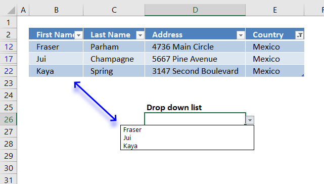
This article demonstrates how to populate a drop down list with filtered values from an Excel defined Table.
The animated image below demonstrates how values (First Name) in a drop down list changes based on how the table is filtered (Country).

How to build this
First we need to insert a new worksheet, this new worksheet will contain a formula that extracts filtered values from the Excel defined Table.
The drop-down list contains a named range that will fetch the extracted values from the new worksheet.
Calculation worksheet
- Press with right mouse button on on any worksheet tab at the very bottom of the Excel screen.
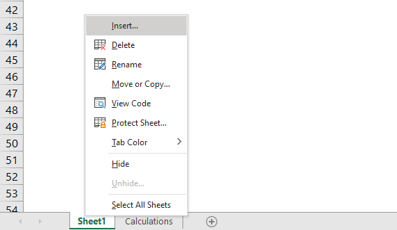
- Press with mouse on "Insert" to open a dialog box.
- Select "Worksheet" icon.
- Press with left mouse button on OK button.
To rename the worksheet simply press with right mouse button on on the worksheet tab and then press with left mouse button on "Rename".
Type a new worksheet name and press Enter, I named it "Calculations".
Formula
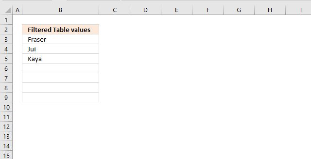
I entered a header name in cell B2.
Formula in cell B3:
- Double press with left mouse button on cell B3.
- Paste above array formula, shortcut CTRL + v.
- Press and hold CTRL and SHIFT keys simultaneously
- Press Enter once
The formula in the formula bar now looks like this: {=formula}
Don't enter these curly parentheses yourself, they appear automatically if you did the above steps correctly.
Explaining formula in cell B3
Step 1 - Create an array
The OFFSET function allows you to identify filtered values if you combine it with the SUBTOTAL function.
OFFSET(Table2[First Name], MATCH(ROW(Table2[First Name]), ROW(Table2[First Name]))-1, 0, 1)
returns {"Kaya"; "Fraser"; ... ; "Kaya"}.
This step may seem weird when you can just use a cell reference to the values, however, that won't work. This step is necessary in order to force the SUBTOTAL function to evaluate each value in the array.
Step 2 - Identify filtered values
The SUBTOTAL function returns 0 (zero) if value is not visible and 1 if the value is visible.
SUBTOTAL(3, OFFSET(Table2[First Name], MATCH(ROW(Table2[First Name]), ROW(Table2[First Name]))-1, 0, 1))
returns {0; 0; 0; 0; 0; 0; 0; 0; 0; 1; 0; 0; 0; 0; 1; 0; 0; 0; 0; 1}
Step 3 - Return row numbers of filtered values
The IF function returns the corresponding row number of each filtered (visible) value and a blank for not visible values.
IF(SUBTOTAL(3, OFFSET(Table2[First Name], MATCH(ROW(Table2[First Name]), ROW(Table2[First Name]))-1, 0, 1)), MATCH(ROW(Table2[First Name]), ROW(Table2[First Name])), "")
returns {""; ""; ""; ""; ""; ""; ""; ""; ""; 10; ""; ""; ""; ""; 15; ""; ""; ""; ""; 20}
Step 4 - Extract the k-th smallest row number
The SMALL function extracts the k-th smallest number in a cell range or array.
SMALL(array, k)
SMALL(IF(SUBTOTAL(3, OFFSET(Table2[First Name], MATCH(ROW(Table2[First Name]), ROW(Table2[First Name]))-1, 0, 1)), MATCH(ROW(Table2[First Name]), ROW(Table2[First Name])), ""), ROWS($A$1:A1))
returns 10.
Step 5 - Return value based on row number
The INDEX function returns a value based on a row number (and column number if needed).
INDEX(Table2[First Name], SMALL(IF(SUBTOTAL(3, OFFSET(Table2[First Name], MATCH(ROW(Table2[First Name]), ROW(Table2[First Name]))-1, 0, 1)), MATCH(ROW(Table2[First Name]), ROW(Table2[First Name])), ""), ROWS($A$1:A1)))
returns "Fraser" in cell B4 which is the 10th value in the array.
The IFERROR function removes errors that will show when there are no more values to show.
Create named range
- Go to tab "Formulas" on the ribbon.
- Press with left mouse button on "Name Manager" button.
- Press with left mouse button on "New.." button to open the Name Manager dialog box.
- Name: Drop_down_list
- Refers to: =INDIRECT("Calculations!$B$3:$B$"&SUMPRODUCT((Calculations!$B:$B<>"")*1)+1)
- Press with left mouse button on OK!
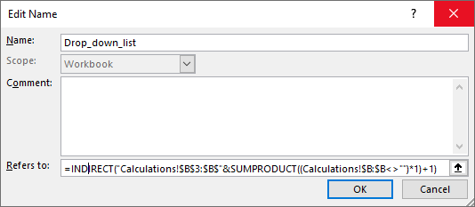
- Press with left mouse button on Close!
Explaining named range formula
The formula used in name range Drop_down_list is dynamic and changes based on the number of values in column B in worksheet "Calculations.
Step 1 - Identify non empty cells in column B
The less and greater than signs combined checks if cells are empty or not.
Calculations!$B:$B<>""
becomes
{""; "Filtered Table values"; "Fraser"; "Jui"; "Kaya"; "" ... ""}<>""
and returns
{"FALSE";"TRUE";... ; "FALSE"}
It is not neccessary to check every cell in column B, if this calculation is slow for you then use a smaller cell reference, for example: Calculations!$B$1:$B$1000<>""
Step 2 - Count non empty cells in column B
The SUMPRODUCT function returns a number representing the total number of non empty cells.
SUMPRODUCT((Calculations!$B:$B<>"")*1)
becomes
SUMPRODUCT({"FALSE";... ; "FALSE"}*1)
The SUMPRODUCT function can't sum boolean values (TRUE or FALSE) so we need to convert them to their numerical equivalents, this is done by multiplying with 1.
SUMPRODUCT({0; 1; 1; 1; 1; 0... ; 0})
and returns 4.
Step 3 - Create cell reference
The ampersand allows you to combine text with a calculation.
"Calculations!$B$3:$B$"&SUMPRODUCT((Calculations!$B:$B<>"")*1)+1
returns
"Calculations!$B$3:$B$5"
Step 4 - Convert text to cell reference
The INDIRECT function lets you use the text as a cell reference.
INDIRECT("Calculations!$B$3:$B$"&SUMPRODUCT((Calculations!$B:$B<>"")*1)+1)
becomes
INDIRECT("Calculations!$B$3:$B$5")
and returns the values in cell range Calculations!$B$3:$B$5.
Create drop down list
- Select cell D26
- Go to tab "Data" on the riboon.
- Press with left mouse button on "Data Validation" button.
- Allow: List
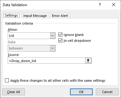
- Source: =Drop_down_list
- Press with left mouse button on Ok
Table category
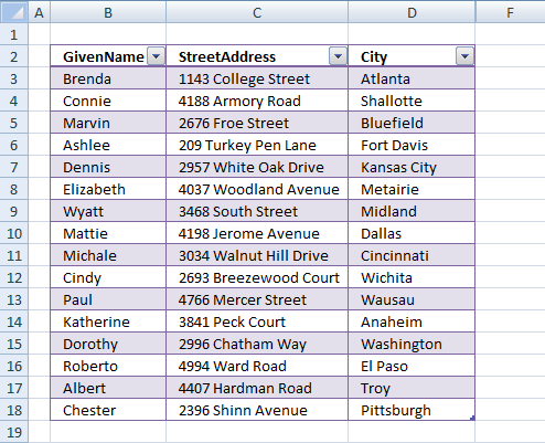
Table of Contents How to compare two data sets - Excel Table and autofilter Filter shared records from two tables […]
This article demonstrates different ways to reference an Excel defined Table in a drop-down list and Conditional Formatting formulas. The […]
The image above demonstrates a macro linked to a button. Press with left mouse button on the button and the […]
Unique distinct values category

First, let me explain the difference between unique values and unique distinct values, it is important you know the difference […]
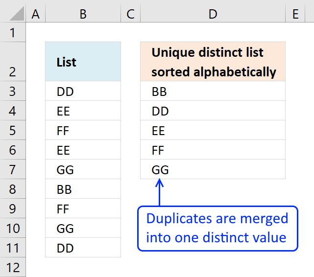
This article demonstrates Excel formulas that allows you to list unique distinct values from a single column and sort them […]
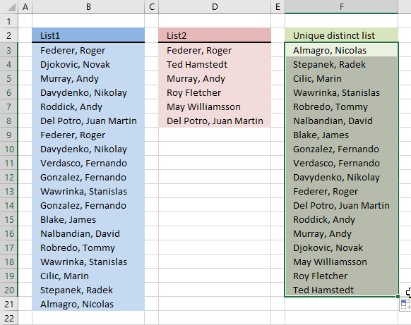
Question: I have two ranges or lists (List1 and List2) from where I would like to extract a unique distinct […]
User defined function category
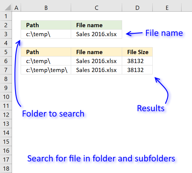
Table of Contents Search for a file in folder and sub folders - User Defined Function Search for a file […]
How to use Excel Tables
31 Responses to “Extract unique distinct values from an Excel Table filtered list”
Leave a Reply
How to comment
How to add a formula to your comment
<code>Insert your formula here.</code>
Convert less than and larger than signs
Use html character entities instead of less than and larger than signs.
< becomes < and > becomes >
How to add VBA code to your comment
[vb 1="vbnet" language=","]
Put your VBA code here.
[/vb]
How to add a picture to your comment:
Upload picture to postimage.org or imgur
Paste image link to your comment.
How do I get the sheet names in a file to becomes the row description in a summary file.
Thxs
Shaz,
Here is an user defined function:
VBA code:
Where to put the code
Press Alt-F11 to open visual basic editor
Press with left mouse button on Module on the Insert menu
Copy and paste the code above
Exit visual basic editor
How to use user defined function
Example,
Select cell A1
Type =List_sheets() in formula bar and then press CTRL + SHIFT + ENTER
Copy cell A1 and paste it to the right
Oscar, what is this line supposed to be doing? I have tried hard to understand this application.caller function, but can't make any sense of it.
iRows = Range(Application.Caller.Address).Rows.Count
appreciate your insight on this.
thanks so much for your tutorials again! They are as always very insightful!
Chrisham,
Thank you!
If you enter the udf in cell range A26:A30, Range(Application.Caller.Address).Rows.Count returns 5.
Application.Caller.Address returns $A$26:$A$30
Its working...! really good solution
Thanks,
Sangam R
It's a nice concept but, when you select Germany in you example, it fails. I think if filtered rows are in consecutive order, it works.
Fowmy,
You are right! It fails, my fault. It looks like it can´t be done without using a helper column. I don´t like "helper" columns. Data Validation lists can´t handle non contiguous ranges.
I even tried creating a named range (and udf) returning a text string using a comma as a delimiter, but that failed too.
I am not sure what to do with this post.
Here is an example file with a "helper" column:
Add-filtered-table-values-to-drop-down-list2.xlsm
The helper column is in sheet2.
I believe that you can get your idea to work if you create a custom function that returns a delimited string from the filtered cell values. Just be sure to credit me :)
David Hager,
I can´t get it to work unless I use a named range. It seems the "drop down list" only accepts a cell range, a named range or a text string.
I used this function:
Function VisibleValues(Rng As Range) As String
Dim Cell As Range
Dim Result As String
For Each Cell In Rng
    If Cell.EntireRow.Hidden = False Then
        Result = Result & Cell.Value & ", "
    End If
Next

VisibleValues = Left(Result, Len(Result) - 2)

End Function
I can only get the custom function to work if I use it in a named range. But then the comma (text delimiter) won´t work. The drop down list shows all values in the same row.
What am I missing?
All credit goes to you :-)
Hi Oscar,
I'm a bit of a newbie trying to learn this and using your formulas and VB above I get an error in the array formulas, it doesn't like the Table2[First Name]. Problem can be that I use Swedish Excel?
I understand that Table2 is the name of the table but [First Name] what does it do and do you know if I need to translate it?
Per,
Problem can be that I use Swedish Excel?
yes, try this formula:
I understand that Table2 is the name of the table but [First Name] what does it do and do you know if I need to translate it?
[First Name] is the first header in the table (col A). Change it to your header name.
[...] Extract unique distinct values from a filtered table (udf and array formula) [...]
Mr. Oscar,
Can i have the values in the blow direction of a cells in udf
"Fraser Horace Jui Kaya Kelton"
Regards
Sudhakar,
I am not sure I understand, try this:
Function FilterUniqueSortTable(rng As Range) Dim ucoll As New Collection, Value As Variant, temp() As Variant Dim iRows As Single, i As Single ReDim temp(0) On Error Resume Next For Each Value In rng If Len(Value) > 0 And Value.EntireRow.Hidden = False Then ucoll.Add Value, CStr(Value) End If Next Value On Error GoTo 0 For Each Value In ucoll temp(UBound(temp)) = Value ReDim Preserve temp(UBound(temp) + 1) Next Value ReDim Preserve temp(UBound(temp) - 1) iRows = Range(Application.Caller.Address).Columns.Count SelectionSort temp For i = UBound(temp) To iRows ReDim Preserve temp(UBound(temp) + 1) temp(UBound(temp)) = "" Next i FilterUniqueSortTable = temp End FunctionDear Oscar,
Thanks for your valuable time, cheers...
Sudhakar
Mr. Oscar,
Fraser Horace Jui Kaya Kelton #N/A #N/A #N/A
Can we eliminate #N/A error from the above udf.
Thanks.
Sudhkar
Sudhakar,
Can we eliminate #N/A error from the above udf.
Yes, I changed the code above.
Mr. Oscar,
Thanks for your help.
Sudhakar
Mr. Oscar,
I have one more question for the same,
Can we eliminate the blank cell or if the cell value is zero in case of alphanumeric sort.
Thanks in advance
Sudhakar
Good Day!
Kindly help me the following issues,
I am in need of a macro instead of “Function FilterUniqueSortTable(rng As Range)” because I have a data in the column say Column A1:A1000, I need to extract the unique value with sort Alpha numerically and put it across columns let us say from B1 to ZZ.
Right now I am using your brilliant function on this thread, its takes a long time when I update the values.
Thanks for your valuable time spend with us
Sudhakar
Somehow the VBA script formula throws a #NAME error for me.
I did the exact copy, just changed the name of the table I want sorted
Id like to make one that is the opposite of what your posted,
ie. the the column gets filtered based on the value you select from a drop down, the drop down is populated with all the unique values of whats present in your table's column
Thanks for referring me to this post, Oscar. This is just what I needed! All I did was change the cell and range references, and I'm in business.
=INDEX(Teachers,MATCH(0,(IF(SUBTOTAL(3, OFFSET(Teachers, MATCH(ROW(Teachers), ROW (Teachers))-1, 0, 1)), MATCH(ROW(Teachers), ROW(Teachers)),""))*COUNTIF($Z$1:Z1,Teachers),0))
Is there a way to have the results display in alphabetical order when the source range (Teachers) isn't?
Rod,
Is it possible to sort the source range?
This formula can do what you ask for but not with filtered values:
https://www.get-digital-help.com/unique-distinct-list-from-a-column-sorted-a-to-z-using-array-formula-in-excel/
No, the source range has to be sorted by a different field. That's OK, I'm happy with what the formula does even without the results being sorted differently than the source. Thanks for your help!
Function VisibleValues(Rng As Range) As String
Dim Cell As Range
Dim Result As String
For Each Cell In Rng
If Cell.EntireRow.Hidden = False Then
Result = Result & Cell.Value & Application.International(xlListSeparator)
End If
Next
VisibleValues = Left(Result, Len(Result) - 2)
End Function
Rüdiger,
Thank you for your contribution.
I had to remove only 1 character to make it work for my example:
Thanks a lot for sharing this. I tried to replicate the formula with the new FILTER() function and it worked.
=FILTER(Table2[First Name],
SUBTOTAL(3, OFFSET(Table2[First Name],
MATCH(ROW(Table2[First Name]), ROW(Table2[First Name]))-1, 0, 1))
)
Oken, thank you for commenting.
It is possible to make your formula even smaller:
To extract unique distinct values use this formula:
Hola
como puedo hacer una consulta , el formulario de contacto no funciona
Gracias
I don't often leave comments when I find a solution to a problem I have had. But your above example for Office365 absolutely solved the problem I was having. You may not need to hear this, but well done - I am very VERY grateful! Thank you!