Extract all rows from a range that meet criteria in one column
I will in this article demonstrate several techniques that extract or filter records based on two conditions applied to a single column in your dataset. For example, if you use the array formula then the result will refresh instantly when you enter new start and end values.
The remaining built-in techniques need a little more manual work in order to apply new conditions, however, they are fast. The downside with the array formula is that it may become slow if you are working with huge amounts of data.
I have also written an article in case you need to find records that match one condition in one column and another condition in another column. The following article shows you how to build a formula that uses an arbitrary number of conditions: Extract records where all criteria match if not empty
This article Extract records between two dates is very similar to the current one you are reading right now, Excel dates are actually numbers formatted as dates in Excel. If you want to search for a text string within a given date range then read this article: Filter records based on a date range and a text string
I must recommend this article if you want to do a wildcard search across all columns in a data set, it also returns all matching records. If you want to extract records based on criteria and not a numerical range then read this part of this article.
What is on this page?
- Extract all rows from a range based on range criteria (Array formula)
- Extract all rows from a range based on range criteria - Excel 365
- Extract all rows from a range based on multiple conditions (Array formula)
- Extract all rows from a range based on multiple conditions - Excel 365
- Extract all rows from a range based on range critera
[Excel defined Table] - Extract all rows from a range based on range critera
[AutoFilter] - Extract all rows from a range based on range criteria
[Advanced Filter] - Get Excel file
1. Extract all rows from a range based on range criteria
[Array formula]
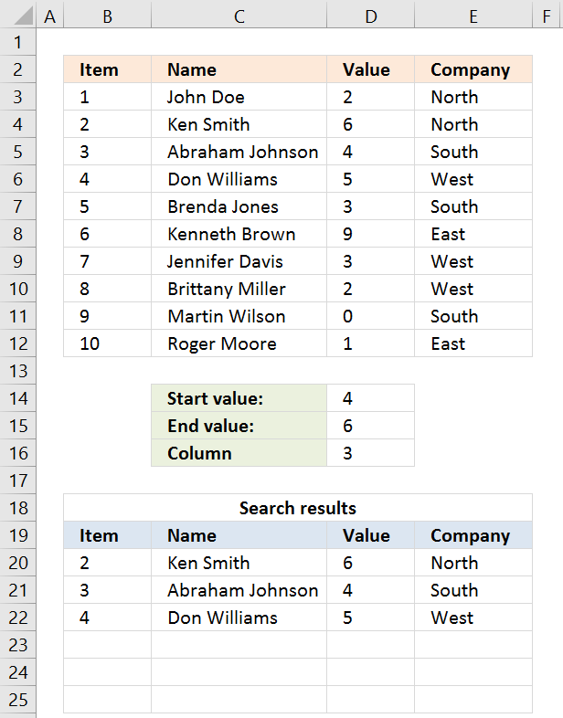
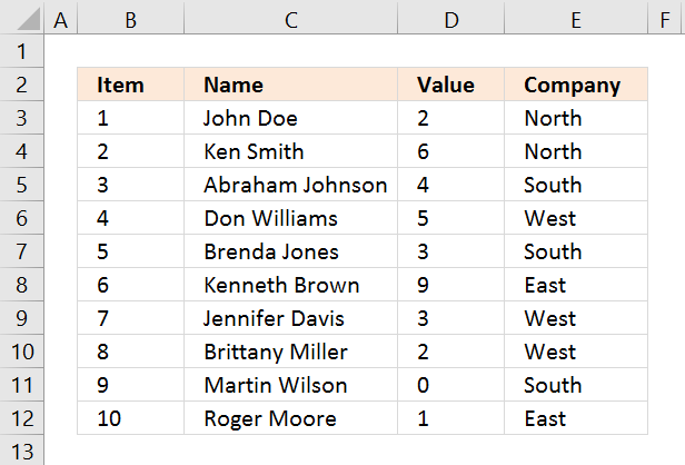
The picture above shows you a dataset in cell range B3:E12, the search parameters are in D14:D16. The search results are in B20:E22.
Cells D14 allows you to specify the start number, and cell D15 is the end number of the range. Cell D16 determines which column to use in cell range B3:E12.
The result is presented in cells B20:E20 and cells below. The example above shows a start value of 4 and an end value of 6, the column is three meaning the third column in cell range B3:E12.
All records that match range 4 to 6 in cell range D3:D12 are extracted, D3:D12 is the third column in B3:E12.
Update 20 Sep 2017, a smaller formula in cell A20.
Array formula in cell A20:
1.1 Video
See this video to learn more about the formula:
[adthrive-in-post-video-player video-id="1tPaXl0I" upload-date="2020-05-26T19:42:56.000Z" name="Extract all rows from a range that meet criteria in one column" description="Filter rows from a range that meet criteria in one column" player-type="default" override-embed="default"]
1.2 How to enter this array formula
- Select cell A20
- Paste above formula to cell or formula bar
- Press and hold CTRL + SHIFT simultaneously
- Press Enter once
- Release all keys
The formula bar now shows the formula with a beginning and ending curly bracket, that is if you did the above steps correctly. Like this:
{=array_formula}
Don't enter these characters yourself, they appear automatically.
Now copy cell A20 and paste to cell range A20:E22.
1.3 Explaining array formula in cell A20
You can follow along if you select cell A19, go to tab "Formulas" on the ribbon and press with left mouse button on the "Evaluate Formula" button.
Step 1 - Filter a specific column in cell range B3:E12
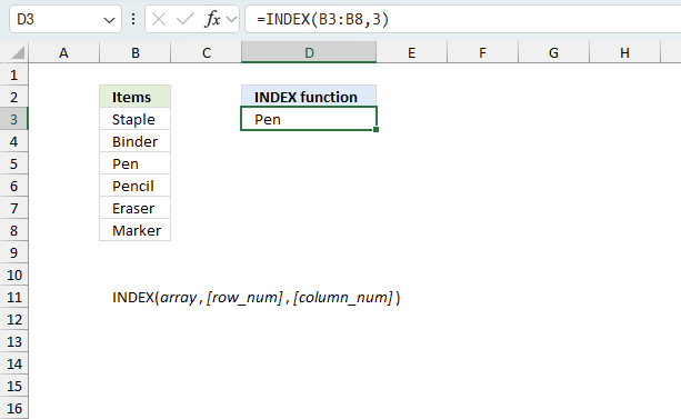
The INDEX function is mostly used for getting a single value from a given cell range, however, it can also return an entire column or row from a cell range.
This is exactly what I am doing here, the column number specified in cell D16 determines which column to extract.
INDEX($B$3:$E$12, , $D$16, 1)
becomes
INDEX($B$3:$E$12, , 3, 1)
and returns C3:C12.
Recommended articles
Gets a value in a specific cell range based on a row and column number.
Step 2 - Check which values are smaller or equal to the condition
The smaller than and equal sign are logical operators that let you compare value to value, in this case, if a number is smaller than or equal to another number.
The output is a boolean value, True och False. Their positions in the array correspond to the positions in the cell range.
INDEX($B$3:$E$12, , $D$16, 1)< =$D$15
becomes
C3:C12< =$D$15
becomes
{2; 6; 4; 5; 3; 9; 3; 2; 0; 1}<=6
and returns
{TRUE; TRUE; TRUE; TRUE; TRUE; FALSE; TRUE; TRUE; TRUE; TRUE}.
Step 3 - Multiply arrays - AND logic
There is a second condition we need to evaluate before we know which records are in range.
(INDEX($B$3:$E$12, , $D$16, 1)< =$D$15)*(INDEX($B$3:$E$12, , $D$16, 1)> =$D$14)
becomes
({2; 6; 4; 5; 3; 9; 3; 2; 0; 1}< =$C$14)*({2; 6; 4; 5; 3; 9; 3; 2; 0; 1}> =$C$13)
becomes
({2; 6; 4; 5; 3; 9; 3; 2; 0; 1}< =3)*({2; 6; 4; 5; 3; 9; 3; 2; 0; 1}> =0)
becomes
{TRUE; FALSE; FALSE; FALSE; TRUE; FALSE; TRUE; TRUE; TRUE; TRUE}*{TRUE; TRUE; TRUE; TRUE; TRUE; TRUE; TRUE; TRUE; TRUE; TRUE}
Both conditions must be met, the asterisk lets us multiple the arrays meaning AND logic.
TRUE * TRUE equals FALSE, all other combinations return False. TRUE * FALSE equals FALSE and so on.
{TRUE; FALSE; FALSE; FALSE; TRUE; FALSE; TRUE; TRUE; TRUE; TRUE} * {TRUE; TRUE; TRUE; TRUE; TRUE; TRUE; TRUE; TRUE; TRUE; TRUE}
returns
{1; 0; 0; 0; 1; 0; 1; 1; 1; 1}.
Boolean values have numerical equivalents, TRUE = 1 and FALSE equals 0 (zero). They are converted when you perform an arithmetic operation in a formula.
Step 4 - Create number sequence
The ROW function calculates the row number of a cell reference.
ROW(reference)
ROW($B$3:$E$12)
returns
{3; 4; 5; 6; 7; 8; 9; 10; 11; 12}.
Step 5 - Create a number sequence from 1 to n
The MATCH function returns the relative position of an item in an array or cell reference that matches a specified value in a specific order.
MATCH(ROW($B$3:$E$12), ROW($B$3:$E$12))
returns
{1; 2; 3; 4; 5; 6; 7; 8; 9; 10}.
Step 6 - Return the corresponding row number
The IF function returns one value if the logical test is TRUE and another value if the logical test is FALSE.
IF(logical_test, [value_if_true], [value_if_false])
IF((INDEX($B$3:$E$12, , $D$16)< =$D$15)*(INDEX($B$3:$E$12, , $D$16)> =$D$14), MATCH(ROW($B$3:$E$12), ROW($B$3:$E$12)), "")
returns
{1; ""; ""; ""; 5; ""; 7; 8; 9; 10}.
Step 7 - Extract k-th smallest row number
The SMALL function returns the k-th smallest value from a group of numbers.
SMALL(array, k)
SMALL(IF((INDEX($B$3:$E$12, , $D$16)< =$D$15)*(INDEX($B$3:$E$12, , $D$16)> =$D$14), MATCH(ROW($B$3:$E$12), ROW($B$3:$E$12)), ""), ROWS(B20:$B$20))
returns 1.
Step 8 - Return the entire row record from the cell range
The INDEX function returns a value from a cell range, you specify which value based on a row and column number.
INDEX(array, [row_num], [column_num])
INDEX($B$3:$E$12, SMALL(IF((INDEX($B$3:$E$12, , $D$16)< =$D$15)*(INDEX($B$3:$E$12, , $D$16)> =$D$14), MATCH(ROW($B$3:$E$12), ROW($B$3:$E$12)), ""), ROWS(B20:$B$20)), COLUMNS($A$1:A1))
returns {2, "Ken Smith", 6, "North"}.
Recommended articles
This article demonstrates how to extract records/rows based on two conditions applied to two different columns, you can easily extend […]
Question: I second G's question: can this be done for more than 3? i.e. (Instead of last name, middle, first) […]

Question: I have a list and I want to filter out all rows that have a value (Column C) that […]
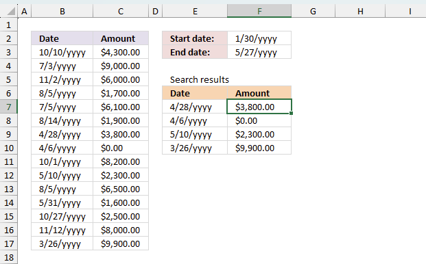
This article presents methods for filtering rows in a dataset based on a start and end date. The image above […]
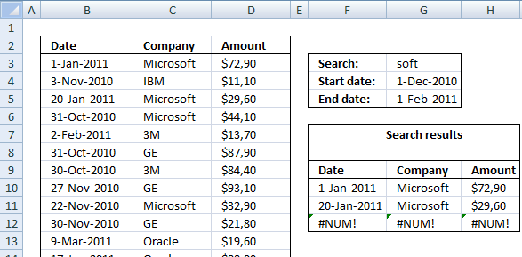
Murlidhar asks: How do I search text in cell and use a date range to filter records? i.e st.Dt D1 […]
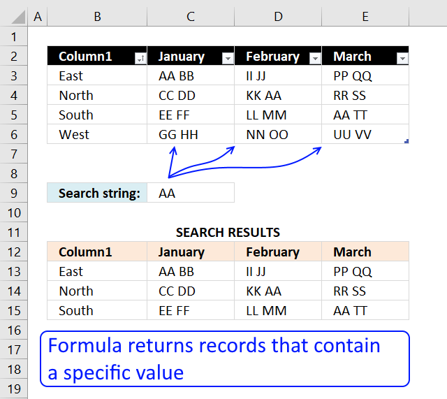
This article explains different techniques that filter rows/records that contain a given text string in any of the cell values […]
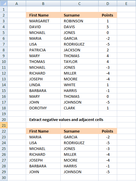
Table of Contents Extract negative values and adjacent cells (array formula) Extract negative values and adjacent cells (Excel Filter) Array […]
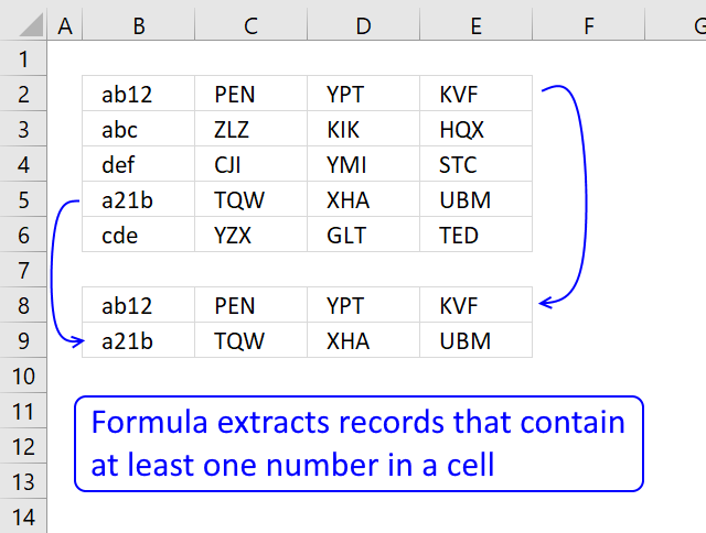
This article describes a formula that returns all rows containing at least one digit 0 (zero) to 9. What's on […]
2. Extract all rows from a range based on range criteria - Excel 365
Update 17 December 2020, the new FILTER function is now available for Excel 365 users.
Excel 365 dynamic array formula in cell B20:
It is a regular formula, however, it returns an array of values and extends automatically to cells below and to the right. Microsoft calls this a dynamic array and spilled array.
The array formula below is for earlier Excel versions, it searches for values that meet a range criterion (cell D14 and D15), the formula lets you change the column to search in with cell D16.
This formula can be used with whatever dataset size and shape. To search the first column, type 1 in cell D16. This is a great improvement in both formula size and how easy it is to enter the formula, compared to the array formula in section 1.
2.1 Explaining array formula
Step 1 - First condition
The less than character and the equal sign are both logical operators meaning they are able to compare value to value, the output is a boolean value.
In this case, the logical expression evaluates if numbers in D3:D12 are smaller than or equal to the condition specified in cell D15.
D3:D12<=D15
becomes
{2;6;4;5;3;9;3;2;0;1}<=6
and returns
{TRUE; TRUE; TRUE; TRUE; TRUE; FALSE; TRUE; TRUE; TRUE; TRUE}.
Step 2 - Second condition
The second condition checks if the number in D3:D12 are larger than or equal to the condition specified in cell D14.
D3:D12>=D14
becomes
{2;6;4;5;3;9;3;2;0;1}>=4
and returns
{FALSE; TRUE; TRUE; TRUE; FALSE; TRUE; FALSE; FALSE; FALSE; FALSE}.
Step 3 - Multiply arrays - AND logic
The asterisk lets you multiply a number to a number, in this case, array to array. Both arrays must be of the exact same size.
The parentheses let you control the order of operation, we want to evaluate the comparisons first before we multiply the arrays.
(D3:D12<=D15)*(D3:D12>=D14)
returns
{0; 1; 1; 1; 0; 0; 0; 0; 0; 0}.
AND logic works like this:
TRUE * TRUE = TRUE (1)
TRUE * FALSE = FALSE (0)
FALSE * TRUE = FALSE (0)
FALSE * FALSE = FALSE (0)
Note that multiplying boolean values returns their numerical equivalents.
TRUE = 1 and FALSE = 0 (zero).
Step 4 - Filter values based on the array
The FILTER function lets you extract values/rows based on a condition or criteria.
FILTER(array, include, [if_empty])
FILTER($B$3:$E$12, (D3:D12<=D15)*(D3:D12>=D14))
returns
{2, "Ken Smith", 6, "North"; 3, "Abraham Johnson", 4, "South"; 4, "Don Williams", 5, "West"}.
3. Extract all rows from a range that meet the criteria in one column [Array formula]
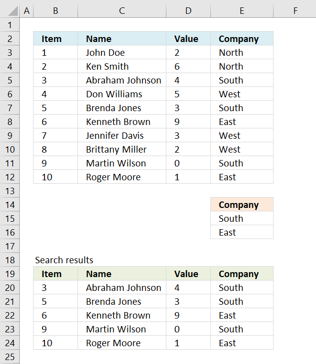
The array formula in cell B20 extracts records where column E equals either "South" or "East". You can use as many conditions as you like as long as you adjust the cell reference $E$15:$E$16 accordingly in the formula below.
The following array formula in cell B20 is for earlier Excel versions than Excel 365:
To enter an array formula, type the formula in a cell then press and hold CTRL + SHIFT simultaneously, now press Enter once. Release all keys.
The formula bar now shows the formula with a beginning and ending curly bracket telling you that you entered the formula successfully. Don't enter the curly brackets yourself.
3.1 Explaining formula in cell B20
Step 1 - Filter a specific column in cell range $A$2:$D$11
The COUNTIF function allows you to identify cells in range $E$3:$E$12 that equals $E$15:$E$16.
COUNTIF($E$15:$E$16,$E$3:$E$12)
returns
{0;0;1;0;1;1;0;0;1;1}.
Step 2 - Return corresponding row number
The IF function has three arguments, the first one must be a logical expression. If the expression evaluates to TRUE then one thing happens (argument 2) and if FALSE another thing happens (argument 3).
The logical expression was calculated in step 1 , TRUE equals 1 and FALSE equals 0 (zero).
IF(COUNTIF($E$15:$E$16,$E$3:$E$12), MATCH(ROW($B$3:$E$12), ROW($B$3:$E$12)), "")
returns
{""; ""; 3; ""; 5; 6; ""; ""; 9; 10}.
Step 3 - Find k-th smallest row number
SMALL(IF(COUNTIF($E$15:$E$16,$E$3:$E$12), MATCH(ROW($B$3:$E$12), ROW($B$3:$E$12)), ""), ROWS(B20:$B$20))
returns 3.
Step 4 - Return value based on row and column number
The INDEX function returns a value based on a cell reference and column/row numbers.
INDEX($B$3:$E$12, SMALL(IF(COUNTIF($E$15:$E$16,$E$3:$E$12), MATCH(ROW($B$3:$E$12), ROW($B$3:$E$12)), ""), ROWS(B20:$B$20)), COLUMNS($B$2:B2))
returns 3 in cell B20.
Recommended articles
This article demonstrates how to extract records/rows based on two conditions applied to two different columns, you can easily extend […]
Question: I second G's question: can this be done for more than 3? i.e. (Instead of last name, middle, first) […]
Question: I have a list and I want to filter out all rows that have a value (Column C) that […]
This article presents methods for filtering rows in a dataset based on a start and end date. The image above […]
Murlidhar asks: How do I search text in cell and use a date range to filter records? i.e st.Dt D1 […]
This article explains different techniques that filter rows/records that contain a given text string in any of the cell values […]
Table of Contents Extract negative values and adjacent cells (array formula) Extract negative values and adjacent cells (Excel Filter) Array […]
This article describes a formula that returns all rows containing at least one digit 0 (zero) to 9. What's on […]
4. Extract all rows from a range based on multiple conditions - Excel 365
Update 17 December 2020, the new FILTER function is now available for Excel 365 users.
Excel 365 dynamic array formula in cell B20:
It is a regular formula, however, it returns an array of values. Read here how it works: Filter values based on criteria
The formula extends automatically to cells below and to the right. Microsoft calls this a dynamic array and spilled array.
4.1 Explaining array formula
Step 1 - Check if values equal criteria
The COUNTIF function calculates the number of cells that meet a given condition.
COUNTIF(range, criteria)
COUNTIF($E$15:$E$16,$E$3:$E$12)
returns
{0; 0; 1; 0; 1; 1; 0; 0; 1; 1}.
Step 2 - Filter records based on array
The FILTER function lets you extract values/rows based on a condition or criteria.
FILTER(array, include, [if_empty])
FILTER($B$3:$E$12, COUNTIF(E15:E16, E3:E12))
returns
{3, "Abraham Johnson", 4, "South"; 5, "Brenda Jones", 3, "South"; 6, "Kenneth Brown", 9, "East"; 9, "Martin Wilson", 0, "South"; 10, "Roger Moore", 1, "East"}.
5. Extract all rows from a range that meet the criteria in one column [Excel defined Table]
The image above shows a dataset converted to an Excel defined Table, a number filter has been applied to the third column in the table.
Here are the instructions to create an Excel Table and filter values in column 3.
- Select a cell in the dataset.
- Press CTRL + T
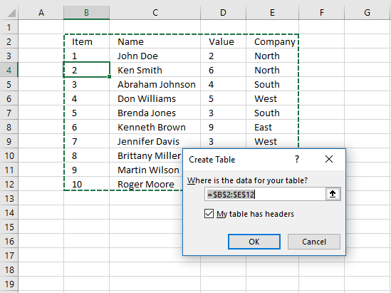
- Press with left mouse button on check box "My table has headers".
- Press with left mouse button on OK button.

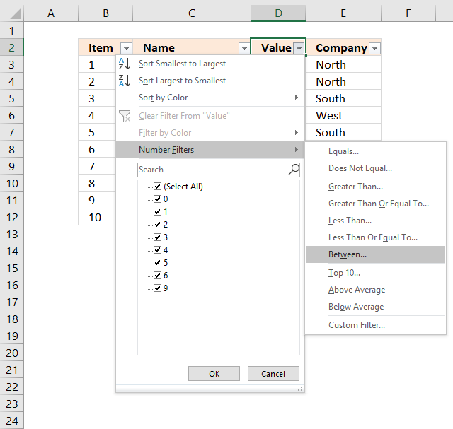
The image above shows the Excel defined Table, here is how to filter D between 4 and 6:
- Press with left mouse button on black arrow next to header.
- Press with left mouse button on "Number Filters".
- Press with left mouse button on "Between...".
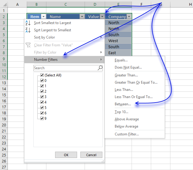
- Type 4 and 6.

- Press with left mouse button on OK button.
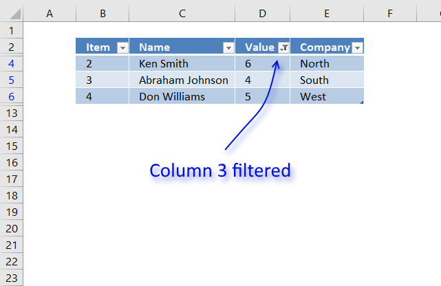
6. Extract all rows from a range that meet the criteria in one column [AutoFilter]
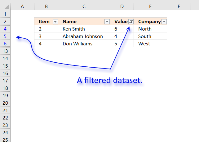
The image above shows filtered records based on two conditions, values in column D are larger or equal to 4 or smaller or equal to 6.
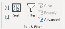
Here is how to apply Filter arrows to a dataset.
- Select any cell within the dataset range.
- Go to tab "Data" on the ribbon.
- Press with left mouse button on "Filter button".
Black arrows appear next to each header.
Lets filter records based on conditions applied to column D.
- Press with left mouse button on the black arrow next to the header in Column D, see the image below.
- Press with left mouse button on "Number Filters".
- Press with left mouse button on "Between".
- Type 4 and 6 in the dialog box shown below.
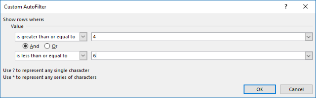
- Press with left mouse button on OK button.
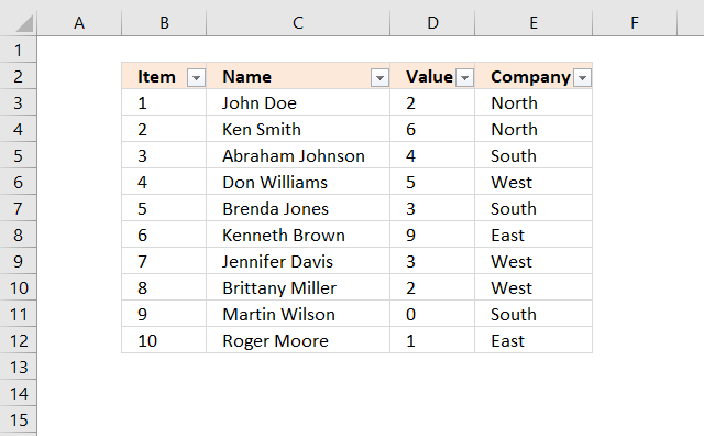
7. Extract all rows from a range that meet the criteria in one column
[Advanced Filter]
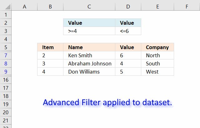
The image above shows a filtered dataset in cell range B5:E15 using Advanced Filter which is a powerful feature in Excel.
Here is how to apply a filter:
- Create headers for the column you want to filter, preferably above or below your data set.
Your filters will possibly disappear if placed next to the data set because rows may become hidden when the filter is applied. - Select the entire dataset including headers.
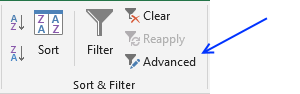
- Go to tab "Data" on the ribbon.
- Press with left mouse button on the "Advanced" button.
- A dialog box appears.
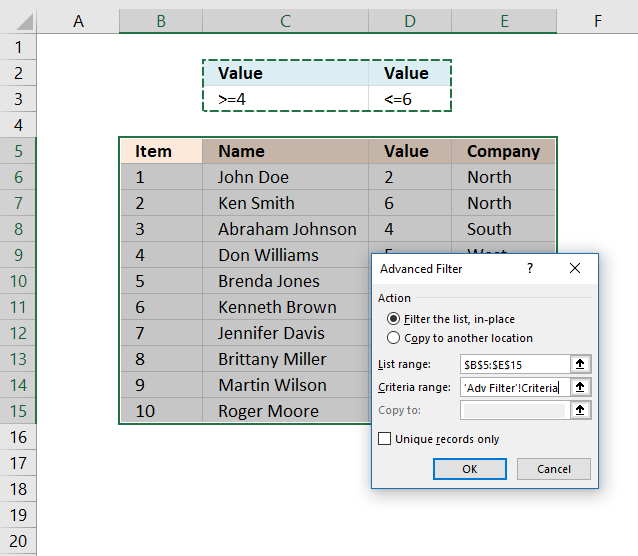
- Select the criteria range C2:D3, shown ithe n above image.
- Press with left mouse button on OK button.
Recommended articles
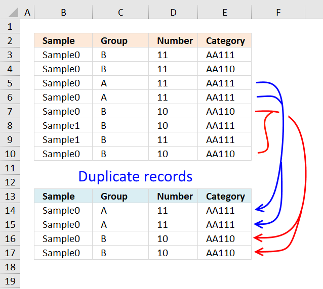
This article describes how to filter duplicate rows with the use of a formula. It is, in fact, an array […]
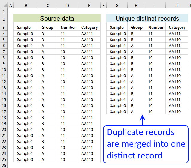
Table of contents Filter unique distinct row records Filter unique distinct row records but not blanks Filter unique distinct row […]
8. Excel file
Filter records category
This article explains different techniques that filter rows/records that contain a given text string in any of the cell values […]
This article demonstrates how to extract records/rows based on two conditions applied to two different columns, you can easily extend […]
This article presents methods for filtering rows in a dataset based on a start and end date. The image above […]
Excel categories
127 Responses to “Extract all rows from a range that meet criteria in one column”
Leave a Reply
How to comment
How to add a formula to your comment
<code>Insert your formula here.</code>
Convert less than and larger than signs
Use html character entities instead of less than and larger than signs.
< becomes < and > becomes >
How to add VBA code to your comment
[vb 1="vbnet" language=","]
Put your VBA code here.
[/vb]
How to add a picture to your comment:
Upload picture to postimage.org or imgur
Paste image link to your comment.
There appears to be an error in your formula.
Row 2 of the list has values of North, 1, 1
The "1" falls in the extract range but it is not included in the results.
Thank you!
I have updated the array formula and the attached file.
this is very very useful, and thanks so much.
q: how would i change the formula, if the "ITEM" is in column A, the "VALUE" is in column B and the "COMPANY" is in column C?
and what is i have another column "NAME" in between columns and ITEM and VALUE
James,
see this blog post: https://www.get-digital-help.com/extract-all-rows-from-a-range-that-meet-criteria-in-one-column-in-excel/
No need for array formulas. Extracting rows that match certain criteria would probably be better done by an advanced filter.
Yes, probably.
There are a lot of steps to create an advanced filter. Doing this multiple times might be timeconsuming? Creating an array formula can also be timeconsuming but when in place only two cell values (C14 and C15) need to be changed to create a new search.
The above array formula is quite small and can be used with a range of any size and shape.
I might be wrong, what do you think?
How does this work if the value you are looking for is a date? For example, I am trying to return rows whose dates match my search criteria. Also, why select rows A1 for the small formula for the "k" value when theres nothing in the cell. Whenever I try it i get a number error.
Hi - I have tried to follow your solution above however only the first record that matches the criteria is displayed over and over again - can you think of what i might be doing wrong?
Hi - bit more clarity - when i got your example, I highlighted the search results section and pressed Ctril + Shift + Enter and the same error came up?
John,
1. Select A19:D19
Copy the array formula to A19:D19 into the formula field + CTRL + SHIFT + Enter , in the example above.
2. Select A19:D19
3. Copy (Ctrl + C)
4. Select B19:D25
5. Paste (Ctrl + V)
Copying cells changes relative references in formulas.
Here is an excellent explanation of absolute and relative references:
https://www.cpearson.com/excel/relative.aspx
Is it possible to have the data on one sheet and the sorted information on another sheet using this formula?
Paul,
Yes!
See file!
Extract all rows that contain a value between this and that.xlsx
Thanks thats great. Is it possible to sort the data in the array eg if the search criteria was dates, nearest dates first. If not how can I copy the data from the array to sort using sort and filter.
Thank you very much!
Paul,
How to copy data from the array
1. Select the cell range
2. Copy (Ctrl + c)
3. Press with right mouse button on a destination cell
4. Press with left mouse button on "Paste Special..."
5. Press with left mouse button on "Values"
6. Press with left mouse button on the OK button!
Now you can sort and filter copied values!
I am trying to get this to work with about 3x the columns that you have here, up to the third column it works as it's supposed to but after the third column it continues to display the first columns name, the same as Johns problem instead of displaying the number that column should contain.. any help?
Hello David,
Did you get a reply on this I am experiencing the same problem.
Thank you
The formulas themselves look exactly the same going across the row, but what is displayed doesnt work..
Hello,
i know this post is very old. but did you get an answer for this?
george,
The formulas themselves look exactly the same going across the row, but what is displayed doesn't work..
No, the formula changes as you copy the cell (not the formula) and paste to cell range B20:E22.
I have bolded the part that changes automatically because of the use of relative cell references:
=INDEX($B$3:$E$12, SMALL(IF((INDEX($B$3:$E$12, , $D$16)<=$D$15)*(INDEX($B$3:$E$12, , $D$16)>=$D$14), MATCH(ROW($B$3:$E$12), ROW($B$3:$E$12)), ""), ROWS(B20:$B$20)), COLUMNS($A$1:A1))
Oscar, how do i get the formulas in cell e21 thru h21 to read the data from cells e3 thru h3? thanks. the current data displayed correctly is in a21 thru d21. I attached a file yesterday using the form.
George,
Oscar, how do i get the formulas in cell e21 thru h21 to read the data from cells e3 thru h3? thanks. the current data displayed correctly is in a21 thru d21. I attached a file yesterday using the form.
I have replied to your email.
Sorry for the confusion, I realized that the attached file was an old file. I have now uploaded a new workbook that better demonstrates the formula in this post.
Does anyone know of a function that can list data from cells relating to a certain criteria?
Here's what I'm trying to do:
On sheet 1 I have a spreadsheet containing publications with various columns for each publication such as title, author, topics covered etc. Each publication is given a reference number.
On sheet 2 I want to create a list by author where it automatically lists the publications (by reference number), that s/he appears in, within one cell.
Oscar perhaps you could help?
@Dan,
If I am reading your question correctly, I believe the UDF (user defined function) I posted in my mini-blog article here will do what you want...
https://www.excelfox.com/forum/f22/lookup-value-concatenate-all-found-results-345/
Hi,
Could you help me so have the results in another sheet (eg: Sheet2). When I tried, getting an error "You Cannot change part of an array".
Thanks
How would I tweak the above formula to look at 2 criteria? In the example above say I wanted the value = 3 AND the company to = south.
My exact problem is I have a data sheet of all invoices for our company. Column headings include customer, invoice number, PO Number, units sold, open/closed, ect. So on a separate sheet I have the formula set up so that based on a drop down you can select the customer, and from there it pulls all invoices from my data sheet. My question is how do I tweak the formula to look at both my customer column and the open/closed column. So I want to be able to see the customers with open invoices. The two cells filled with yellow are my input cells and are the criteria for my table below. You can see based on the yellow box with “AAA Sales” selected, my table is returning the correct customer but now I want only open invoices.
https://postimg.org/image/k012ex1ih/
John Cejka,
Get the Excel *.xlsx file
Extract-all-rows-that-contain-a-value-between-this-and-that-part-21-John-Cejka.xlsx
Thanks Oscar, that is what I need and it works perfectly on your sheet, but I cannot copy and or paste the formula, or even manually type it. I think it has something to do with the fact that on your sheet I see { at the beggining and } at the end of your formula. Any suggestions?
Your formula and template work fantastic. I am having one issue that I have spent more time than I wish to say on trying to alter it, to no avail. What I need to do is expand the amount of columns it pulls. I need it to pull 2 in front (to the left) of the search number and 7 after (to the right) of the search number. The immediate 2 columns to the right of the searched number is actually hidden and not used, but I wasn't sure if it would make it to complicated to pull the 5 after the 2 hidden. Please help. Thanks in advance.
I use filters like this every day, there's a really simple way to hide all rows that have a certain value in one column: Simply add filters to every column.
> Don't select any cells - just press with left mouse button on one in the middle of your spreadsheet somewhere.
> Hit Ctrl+Shift+L (You should see drop down arrows appear at the top of every column - if you don't have column headers you will want to put some in, otherwise your first row of data will be treated like column headers.)
> Go to the column with the data you're trying to remove, press with left mouse button on the drop down, and uncheck that data in the list.
> All rows containing that data will be automatically hidden.
Jason,
Yes, filters are very useful.
Thank you for commenting!
thanks a lot for this, do you have an example where need to check for 2 conditions?, many thanks!!
Using this as an example I want to extract all records with Company = East and place those records in sheet 2. Can you show me how to do that?
Ultimately I want to have multiple sheets showing subsets of records from sheet 1 that match a text criteria. So again, using this example, sheet 2 would show all records for Company = East, sheet 3 would have all records for company = West, etc.
=IF(ISERROR(INDEX(EOD.xlsx!$A$1:$I$1648,SMALL(IF(AND(EOD.xlsx!$I$1:$I$1648>=40000,EOD.xlsx!$I$1:$I$1648=40000,EOD.xlsx!$I$1:$I$1648=40000), it gives the desired result , BUT while using AND operator(to match if the value is greater than or less than), it doesn't give desired results. What am I doing wrong here?
=IF(ISERROR(INDEX(EOD.xlsx!$A$1:$I$1648,SMALL(IF(AND(EOD.xlsx!$I$1:$I$1648>=40000,EOD.xlsx!$I$1:$I$1648=40000,EOD.xlsx!$I$1:$I$1648<50000),ROW(EOD.xlsx!$I$1:$I$1648)),ROW(1:1)),1))
When I use single condition, it gives the desired results BUT while using AND operator(to match if the value is greater than or less than), it doesn't give desired results. What am I doing wrong here?
[…] = window.adsbygoogle || []).push({}); Dear friends, I found this site (Extract all rows from a range that meet criteria in one column in excel | Get Digital Help - Microso…) with a very good formula and very helpful for my task that I have to complete. I attached these […]
Hi,
First: I´ve been analyzing your formula since it could be very useful in a worksheet I´m working, and using the exact same format, I found that it doesn´t work. When pressing CTRL+SHIFT+ENTER, I get a message "You´ve entered to many arguments for this function." I changed the comas for semi-colens, and yet the error persists.
On the other hand, how did you limit to a maximum of 3 (cell F2), this cell doesn´t appear in your formula.
Thanks for the help.
if i have a range of values and i am asked to display values greater than a specific value only,what do i do?
daniel,
Use this formula:
=INDEX(tbl, SMALL(IF((INDEX(tbl, , $C$15, 1)<=$C$14), ROW(tbl)-MIN(ROW(tbl))+1, ""), ROWS(A19:$A$19)), , 1)
I have been trying to make this code work for me but I am at a total loss. I have Colomn C and when it turns to GA (through an IF Function) I would like excel to copy the row and paste it into another sheet in the file. How can I accomplish this.
Good day
I have table 1
Jan Feb Mar Apr May Jun
Ben 1 1
Ben 1
Ben 1
Rick 1
Rick 1
Rick
then I have Table 2
Jan Feb Mar Apr May Jun
Ben
Rick
I need a formula in table 2 that will look in table 1
and bring back the number 1 for Ben under Jan , Feb , May and June
and the same for Rick under Mar and Apr
thanks
Hello.
I have a drop down list in column H. Values = A, B and C
I would like to have a dynamic column I, whereby, if I select 'A' in column H, than a defined list would be presented in the cell next to it. If I select 'B', a different predefined list would be presented.
Any help would be greatly appreciated.
it doesn't work if the range is as C2:F30000. The formula return REF error.
How can I fix it ?
Andrea,
Can you post your formula?
Hi Oscar
Your solution/ formula is fantastic. I tried to modify it to my range but it only extracts the first four columns only.
Hence I added one more col. to your sheet (thinking that I might be doing something wrong)but here to it only copies the first four cols only.
What I did was ( in the result area) copied formula from D19 to E19 but it extracted the value from col A instead from from col E.
Please let me know what I am doing wrong.
Many thanks
I have the exact same problem. It only works for 4 columns. When I try to put an additional column to the right I get the values of the 1st column instead of the 5th.
can i have the option not to display #num! error message. display blank or "-"?
Hi How do I get rid of the #NUM and show a blank please?
how to extract opposite?
a given date through a range of dates: B1 lower date, c1 higher date
only values where given date, ex $d$10, is between b1 and c1
extract a1....
Hi,
I tried to copy and paste the formula and adjust it for my use, but it's not returning what I would expect - instead it's returning a single row from the tale that is outside of my range...
I feel like I could guess the logic for most of the inputs, except for the match part of the function, so I feel like that may be a key reason for why it's not working for me. Could someone please explain the logic behind the inputs of the Match function to me (and how that impacts the results of the function small)? Or if someone is willing to share what they did in hopes that I can compare the examples and figure out what I need to change...
Thanks
I've figured out the logic behind the functions and inputs...but for some reason, while I can copy and paste the cells, the minute I try either editing the cells I get an error. I feel like it might be that while the original is somehow able to evaluate into an array of T/F, or {1,....,n} when I try to write the formula it will try to condense the T/F arrays into a single value and/or have issues with dimensions/orientations of the array values. Anyone know of a way to fix this?
You need to use the IFERROR function
=IFERROR(INSERT YOUR CODE HERE,"")
Hi, I am trying to use this code to copy rows to a different sheet column 4 must equal "A". i dont want to use the 3 range cells C13,14 &15 to set the criteria. i have named my source table tbl same as above and is located in sheet1 and i want to copy all the rows that meet the criteria to sheet2.
thank you
Stephen, you don't have to use a formula to extract records where column 4 is equal to A.
1. Select the range you want to filter
2. Go to tab "Home" on the ribbon
3. Press with left mouse button on "Sort & Filter" button
4. Press with left mouse button on the arrow in column 4 and only select "A"
Now you can copy filtered rows to sheet2.
However, if you do want to use a formula this post describes how to:
https://www.get-digital-help.com/how-to-return-multiple-values-using-vlookup-in-excel/#multiple
Remember to change the cell ref to column 4 in the formula.
Hi,
I am trying to modify this formula so that I display only the rows where the value in the '$C$15' column are blank. What do I do?
Hi Oscar
This is an excellent solution that does not require data refresh like power query.
I modified your query to match two values which suits my requirement: {=IFERROR(INDEX(Data,SMALL(IF(($G$1=Value1)*($G$2=Value2),MATCH(ROW(Item),ROW(Item))),ROW(A1)),COLUMN(A1)),"")"
I am trying to understand the purpose of the Item column. Changing the values in this column does not seem to affect the result.
Thanks
Hi Arthur
Thank you.
I am trying to understand the purpose of the Item column. Changing the values in this column does not seem to affect the result.
If you are asking why I use the Item column in the formula the answer is that I use the range to create numbers for each row. As long as the Item column has as many rows as the Data column you can use both (not at the same time), it doesn't matter.
Hi Oscar
Really love your approach.
I added one more column......but....the data on my 5th column gives the results of the first column...
I know you have been asked many a times...i read carefully what you replied...but its still does not work...
Please Please help.
thanks
Oscar:
Thanks very much for this tutorial! It has been VERY helpful. However, I must be doing something incorrectly. I have been able to get to a certain point, but I cannot get the formula to return the data in subsequent columns. As I copy the formula across (from column A to B to C, etc.), it just keeps repeating the data from my very first column. Any suggestions would be greatly appreciated!
Peter,
My guess is that the cell ref in your column() function is an absolute cell ref?
Is your formula entered as an array formula? Can you see a beginning and ending curly bracket, like this: {=array_formula} in the formula bar?
Nice website..am glad i have learned lots of stuff .Av managed to complete my excel vba accounting software.keep it up...Dedan frok Kenya
if i have 3 range of values and i am asked to display that 1st condition is equal to specific value, 2nd condition not equal to specific value only, extract row based all values without repeat what do i do?
repeat x times based on cell value and based on condition
Hi Oscar! I like your stuff very much but this formula can't seem to work for me. It returns #N/A's..
{=IF((INDEX($A$2:$D$11, , $C$15, 1)=$C$13), MATCH(ROW($A$2:$D$11), ROW($A$2:$D$11)), "")}
Also, why are you using $A$2:$D$11 as array? Shouldn't it be $B$3:$E$12?
Thanks
Hi Martin
this formula can't seem to work for me. It returns #N/A's..
Did you enter the formula as an array formula?
Also, why are you using $A$2:$D$11 as array? Shouldn't it be $B$3:$E$12?
Yes, the explanation uses $A$2:$D$11 but it should be $B$3:$E$12. I have updated the article.
Sorry for the confusion.
Oscar i freaking love you right now. You helped me solve the issue with my spreadsheet that i have been struggling with for a week.
Alec
Thank you, I am happy I could help you out.
I feel like I could figure the rest of this out, but I still don't understand how, in the first example, when he is extending down the index formula (right around the 3:10 mark), it is not just returning the first result over and over. I see other people have asked, and he responded regarding absolute vs relative, but I don't see how that would apply, since in his example, he is using absolute references on all the cell references.
Can Oscar or someone else explain in another way? I'm really lost.
Hi Tim
he is using absolute references on all the cell references.
Not all cell references, this part of the formula is different:
ROWS(B20:$B$20)), COLUMNS($A$1:A1))
The first part is absolute and the second part of the cell reference is relative or vice versa.
What if you have this data (table data) and you need to get the Total stone wt. (highlighted in blue box)(pls. Press with left mouse button on link for the screenshot https://postimg.cc/image/mlu9yty93/) How would you formulate it for Index Match? Is it possible to get the desired result?
Let me know. Thanks.
Aiz
Sorry if I don't understand.
Why can't you use the SUM function?
Hi ,
I have the data in below format:
A -100
B -234
C -32
A -123
B -221
D -456
A -145
B -245
C -312
D -478
I want to format this data as:
A B C D
100 234 32
123 221 456
145 245 312 478
Could you please help me how it can be done in excel?
Regards,
Neeraj Sharma
Hi Oscar - Thanks for this amazing formula. Really appreciate the clear explanation on the video.
Tribhuvan Gupta,
thank you!
Hi I have one GRN no ex: GRN1 and this will be having one Invoice number i.e 123 in this invoice 4 items will be available i,e Item 1 Item 2 Item 3 Item 4 and each item will be having respecting Qty details in master data.
So My question is How can I extract qty details by considering GRN no and Invoice No.
"GRN No and Invoice No will be unique and will not repeat"
Please help me.
MATCH(ROW($B$3:$E$12), ROW($B$3:$E$12))
Could you please explain this part.
I am getting only 1 in all rows or this
Jinson,
MATCH(ROW($B$3:$E$12), ROW($B$3:$E$12)) creates an array {1;2;3;4;5;6;7;8;9;10} used to identify which row to get values from.
I believe you get 1 in all rows because you didn't enter the formula as an array formula. CTRL + SHIFT + ENTER
=IF(FIND(",",C6,1)>0,LEFT(C6,(FIND(",",C6,1)-1)),C6) where there is no comma in cell am getting error
This is a great formula and I've almost solved my issue using it, so thank you! The last piece of my problem requires me to further narrow down the search results using not only one category, but two categories. Is it possible to further narrow down the results to only show one type of company (ie only show results between values of 4 and 6 who's company is called North?
Fotini,
Yes, it is possible.
=INDEX($B$3:$E$12, SMALL(IF((INDEX($B$3:$E$12, , $D$16)<=$D$15)*(INDEX($B$3:$E$12, , $D$16)>=$D$14)*($E$3:$E$12="North"), MATCH(ROW($B$3:$E$12), ROW($B$3:$E$12)), ""), ROWS(B20:$B$20)), COLUMNS($A$1:A1))
Hi,
How do you get the "#NUM!" to hide like in your other table. Is it possible to make it look empty or contain a dash rather than that?
Also thank you! This was very helpful.
DIana,
I use the IFERROR function to catch errors, however, use with caution, it takes all kinds of errors.
=IFERROR(INDEX($B$3:$E$12, SMALL(IF((INDEX($B$3:$E$12, , $D$16)<=$D$15)*(INDEX($B$3:$E$12, , $D$16)>=$D$14), MATCH(ROW($B$3:$E$12), ROW($B$3:$E$12)), ""), ROWS(B20:$B$20)), COLUMNS($A$1:A1)),"")
or a dash:
=IFERROR(INDEX($B$3:$E$12, SMALL(IF((INDEX($B$3:$E$12, , $D$16)<=$D$15)*(INDEX($B$3:$E$12, , $D$16)>=$D$14), MATCH(ROW($B$3:$E$12), ROW($B$3:$E$12)), ""), ROWS(B20:$B$20)), COLUMNS($A$1:A1)),"-")
Oscar,
I wanted to take a moment to say a massive thank you for your work above.
I am relatively a novice and have been struggling for weeks to get something exactly as above.
I will be reading with interest your other articles following this, as I suspect they will all be of equal quality and a great opportunity to expand my own knowledge.
Many thanks again.
MJB.
MJB,
thank you!
This does precisely what I'm wanting to achieve, but how do I implement it using VBA?
Regards,
Ben
How does this work if the value you are looking for is a date? For example, I am trying to return rows whose dates match my search criteria. Also, why select rows A1 for the small formula for the "k" value when theres nothing in the cell. Whenever I try it i get a number error.
Can you use negative values, or how do you exclude values that may be blank?
Tom,
Negative values seem to work?
I have added content to this article regarding excluding values that may be blank.
Thank you for this addition, this site is very informative and helpful. Great Resource!!
Can this same logic be used to obtain list based on multiple criteria?
To clarify, how do you extract row(s) if matching a value and a price?
Oscar,
Quick question. can this exact same spreadsheet work if you remove the item number column? or in other words, can this work if it only has name, value, and company without some numerical way of tracking/identifying each row?
Ross,
Yes, this take a look at this example Extract all rows from a range based on multiple conditions
[Array formula]. Although the example has a item number column you don't have to reference that column in your workbook.
The formula becomes:
=INDEX($C$3:$E$12, SMALL(IF(COUNTIF($E$15:$E$16,$E$3:$E$12), MATCH(ROW($B$3:$E$12), ROW($B$3:$E$12)), ""), ROWS(B20:$B$20)), COLUMNS($B$2:B2))
Hello,
I am trying to extract all rows that contain any text. I have done this, following your example, in the following way:
=LOOKUP(2; 1/((COUNTIF($A$43:A43; 'Raw Data'!$Y$3:$Y$400)=0)*(MMULT(--(ISNUMBER(SEARCH(""; 'Raw Data'!$Y$3:$Y$400))); {1})=1)); 'Raw Data'!$Y$3:$Y$400)
(notice that my Excel is set up so that I must use ; where you would use ,)
This works fine for all strings up to 255 characters. Strings of more than 255 characters do not show up in my list. Is there any way to get around this?
Thank you!
Regards,
Adam
Hi.
I need to create a etoll spreadsheet and am struggling!
I have a report telling me what date was the toll charged and the car plate.
I also have another spreadsheet with customer names, plates of the car they rented, start day of the rental and end day for the rental.
what I need is a Result spreadsheet where I can see: on that date that the toll was charged, who was driving that particular car.
Do you have an easy way of doing this? Tried using your "Match two criteria and return multiple records [Array Formula]" but had no success.
Please help!
Thanks and regards,
Stephany
Hi
For some reason whenever I enter =MATCH(ROW($C$3:$C12),ROW($C$3:$C$12)) verbatim I get an N/A error message. I even tried the file to get it to work, and the numbers were there initially, but after I tried copying the formula the number switched to an error message.
'Object Display Latest Premium Paid Date
'Original Formula in Policy Detail Worksheet ->
' =IFERROR(INDEX(Prem_Pay_Hist[Date of Premium Payment],
' LARGE(
' IF(Prem_Pay_Hist[Policy No]=Pol_details_Policy_no,
' ROW(Prem_Pay_Hist[Date of Premium Payment])-MIN(ROW(Prem_Pay_Hist[Date of Premium Payment]))+1),
' 1)
' ),
' "")
This cell formula works fine but I want to code it in vba
How to code this formula in excel vba
Thanks for this incredible formula! When I use this, it displays 0 for cells where the original data is empty cell. How do I avoid that? And display empty cell as original?
Hi
For some reason whenever I enter =MATCH(ROW($C$3:$C12),ROW($C$3:$C$12)) verbatim I get an N/A error message. I even tried the attached file to get it to work, and the numbers were there initially, but after I tried copying the formula the number switched to an error message.
Is there a non array version for Extract all rows from a range that meet criteria in one column:
=INDEX($B$3:$E$12, SMALL(IF(COUNTIF($E$15:$E$16,$E$3:$E$12), MATCH(ROW($B$3:$E$12), ROW($B$3:$E$12)), ""), ROWS(B20:$B$20)), COLUMNS($B$2:B2))
Appreciate for the help over here. thanks
Can we sort the output, ie the solution return rows/columnw which fall betn two values. My query is whether the output can in ascending/descending order of that value. Eg if we search for values betn 3 & 6 in array {1:5:6:2:3:9:4}, out put will be 5:6:3:4, i require it to be 3:4:5:6 or viceversa
Hi
If all the information comes from one Column A & I have two difference criteria's names, how to retrieve a table between two difference names?
The table varies in row number & there are ten tables to retrieve.
$A$6:$A$300 is the criteria between name range. Helper column BV4 & BV34
$A$6:$J$300 is the table range.
No is start of table heading over ten columns.
1 to 24E is the numbers down table to retrieve. Helper column CL8, CL7 & CL6 for
1, 24E & 0
The formula below is the extract match of the table but table varies?
{=INDEX($A$35:$J$45,SMALL(IF((INDEX($A$35:$J$45,,$CL$8)$CL$6),MATCH(ROW($A$35:$J$45),ROW($A$35:$J$45)),""),ROWS($CM$6:CM6)),COLUMNS($A$34:A34))}
The formula below is the extract match of the criteria but can’t stop & add next table in same table.
{=INDEX($A$6:$J$300, SMALL(IF(COUNTIF($BU$9:$BV$34,$Z$6:$Z$300), MATCH(ROW($A$6:$J$300), ROW($A$6:$J$300)), ""), ROWS($A$6:A6)), COLUMNS(A$6:$A6))}
Any help would be greatly appreciated.
Regards
Tony
Mistake first formula should read
{=INDEX($A$35:$J$45,SMALL(IF((INDEX($A$35:$J$45,,$CL$8)$CL$6),MATCH(ROW($A$35:$J$45),ROW($A$35:$J$45)),""),ROWS($CM$6:CM6)),COLUMNS($A$34:A34))}
I tried to get the excel file and in Dataset - criteria tab when I press the enter key in B20 it becomes #Value. Why is it?
Des, I'm having exactly the same issue. I have a relatively big data set of 18 or so column.
When trying to get the k-th number it returns #Value on the rows to be excluded and #NUM on the rows to be included.
I figured it out. The cell needs to be indexed. F2+Cnrl+Enter
Hi Oscar,
This Function works great for me vertically however, when I drag right or left to capture the other information in the row, I get a reference error and the only change I can spot in in the final Rows and Columns range where it extends.
Do you know why this might be happening and how I can over come this?
My version of the function is:
{=INDEX('1. W2W Tracker'!$F$4:$F$176, SMALL(IF(COUNTIF($B$5:$B$7,'1. W2W Tracker'!$F$4:$F$176), MATCH(ROW('1. W2W Tracker'!$C$4:$K$176), ROW('1. W2W Tracker'!$C$4:$K$176)),""), ROWS($C$5:C5)), COLUMNS($C$5:C5))}
your instruction is very good.
just wondering if i just wanted only > certain value only without the 4 no upper limit do i still have to use small function?
what should the formula be, please advice, thank you.
Hello Oscar,
Thank you a lot for this explanation! I spent almost two days trying to figure out a way to search a way to return multiple matches based on several criteria involving ranges. This was the solution to this.
Thanks again !
Marvy,
thank you for commenting!
Hi
The Array formula does not work for me (when I adapt it).. And specifically the first nested statement is where I trace the issue.. COUNTIF does not match Excel syntax..
From Array Formula Step 1
The COUNTIF function allows you to identify cells in range $E$3:$E$12 that equals $E$15:$E$16.
COUNTIF($E$15:$E$16,$E$3:$E$12)
----the above is in format (criteria, range)
BUT Excel says it should be COUNTIF (range,criteria)
The link highlighted in the example using "Lucy" follows what I say
excelente.
Hello, thank you very much for this! This is really helpful.
However, I tried to use the formule on a lot of data and it does not work. It returns the "number" value.
This is the formule in dutch:
INDEX($AI$17:$AK$35057;SMALL(IF((INDEX($AI$17:$AK$35057;;1)>=$AJ$12)*(INDEX($AI$17:$AK$35057;;1)=$AJ$14)*(INDEX($AI$17:$AK$35057;;2)=$AJ$12)*(INDEX($AI$17:$AK$35057;;1)=$AJ$14)*(INDEX($AI$17:$AK$35057;;2)<=$AJ$15);VERGELIJKEN(RIJ($AI$17:$AK$35057);RIJ($AI$17:$AK$35057));""); RIJEN($A$1:A1));KOLOMMEN($A$1:A1))
Thank you SO very much! I have been working on this for 2 days and never could figure it out. You are an absolute life saver!
Thank you Gwen!
Big Thank you. First approach works great on all Excel versions.
Hi,
I have data in Col E separated with commas like South,East, North. The formula needs to search Col E and export rows if the value matches in E.
Thanks
I want to pull all rows from a table where one of the columns equals a specific text string, I can't figure out how to apply this to my issue.
Louis,
The FILTER function can do that for you.
Here is an example: Extract multiple records based on a condition
Hi,
Thank you for an incredibly useful webpage....
I just had a question though...
Having built a formula to get the details of the row with the nth largest value in a particular column (in this case the nth largest in column P - with nth defined by the value in column A)
=INDEX(Scotland!$B$3:$B$33, MATCH(LARGE(IF(Scotland!$I$3:$I$33="Y",Scotland!$P$3:$P$33), $A89),IF(Scotland!$I$3:$I$33="Y",Scotland!$P$3:$P$33), 0))
This works fine UNTIL I get to where there are duplicate values in column P, and the formula just takes the first one and I get a duplicate in the row.
Is there a way to ensure that it doesn't take the same value twice?
Tim,
You can use the COUNTIF function to prevent duplicates, here is an example:
Extract a list of alphabetically sorted duplicates based on a condition
This part of the formula makes sure it displays only one instance of the duplicate.
COUNTIF($E$4:E4, $C$3:$C$9)=0
I want to extract whole raw from main data to other sheet, if I met certain certeira is met.
Example
S.NO. Gender Subject Score State
1 Male Match 90 New York
2 Female Science 92 Las angeles
3 Male Match 48 Chicago
4 Male Value Education 92 Washington
5 Female Political Sc 64 Las Vegas
How to pull to other worksheet by functions(Not with filter>copy>past) only data of Male
Refer required result as below
S.NO. Gender Subject Score State
1 Male Match 90 New York
3 Male Match 48 Chicago
4 Male Value Education 92 Washington
Please help me to find the function
Thanks
How to extract the whole raw from the data to other worksheet if the creteria met.
My data is follows.
Sl Gender Subject Markes City
1 Male Maths 85 Las Angeles
2 Female Physical Science 69 New York
3 Male Value Education 92 Chicago
4 Female Political Science 75 Washington
5 Male Medical Science 51 Las Vegas
6 Male Business Science 37 Dallas
I want the the values contain second column as "Male" the other work sheet.
Result must be as below
Sl Gender Subject Markes City
1 Male Maths 85 Las Angeles
3 Male Value Education 92 Chicago
5 Male Medical Science 51 Las Vegas
6 Male Business Science 37 Dallas
Sunil Pinto,
The FILTER function is the easiest way, in my opinion.
Hi Oscar...how can the Filter function be used to identify and list rows containing a text string, as listed in a range of text strings eg
*abbotts*
*aldi*capital
*fabrics*capital
*air*filter
*bed*bath*table*
*engine*maint
*deft*maint*
*ikea*capital
I'm using Office 365 but the formula above seems to require a full match
Thanks
Michael Sandy
Michael Sandy,
I think you are looking for this: Filter values if cell contains given string
or this: Display matches if the cell contains text from a list
Hi There,
First off, thank you very much for this it is really useful.
I was wandering if it was possible to work if one of the cells with the value was missing?
e.g. D14 was present with a value of 4, but no D15 value (as it isn't know).
Ultimately I am trying to get this to work so that if some of the criteria I am looking for is not entered it will ignore and look at the next critera.
Is that possible?
Thanks in Advance,
Stephen