Find and return the highest number and corresponding date based on a condition
Table of Contents
- Introduction
- Find and return the highest number and corresponding date based on a condition - Excel 365
- Find and return the highest number and corresponding date based on a condition - Excel 2016
- Find and return the highest number and corresponding date based on a condition
- Lookup value based on two critera – second criteria is the adjacent value and its position in a given list
1. Introduction
Denis asks:
thank you for sharing you knowledge and helping us with these excellent formulas.
I have a case i could really need your help with:
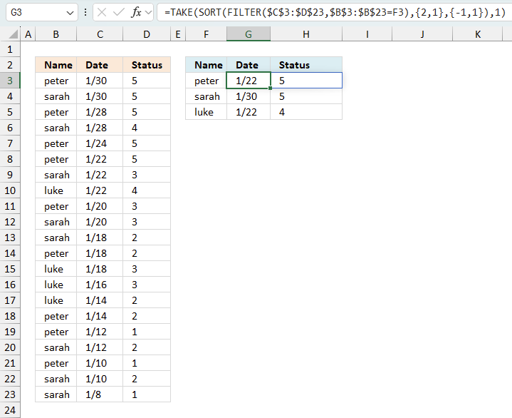
The following Table shows a history of names, stati and the date the status was acquired. BUT: people can acquire the same status more than just once (or at least report it). Now I want to know, when each person (peter, sarah & luke) have acquired their individual highest status.Name Date Status
peter 30.01.2015 5
sarah 30.01.2015 5
peter 28.01.2015 5
sarah 28.01.2015 4
peter 24.01.2015 5
peter 22.01.2015 5
sarah 22.01.2015 3
luke 22.01.2015 4
peter 20.01.2015 3
sarah 20.01.2015 3
sarah 18.01.2015 2
peter 18.01.2015 2
luke 18.01.2015 3
luke 16.01.2015 3
luke 14.01.2015 2
peter 14.01.2015 2
peter 12.01.2015 1
sarah 12.01.2015 2
peter 10.01.2015 1
sarah 10.01.2015 2
sarah 08.01.2015 1answers have to be :
Names latest status in status since
Peter 5 22.01.2015
sarah 5 30.01.2015
luke 4 22.01.2015I would really appreciate your help.
Greetings.
2. Find and return the highest number and corresponding date based on a condition - Excel 365
The following formula returns an Excel 365 dynamic array formula that spills values horizontally.
- It uses the value in column F on the same row to filter the correct rows from cell range B3:D23.
- Sorts the values based on status from high to low.
- Extracts the top row from the array.
Formula in cell G3:
The formula returns both the date and status based on the name specified in column F. This is called spilling and is a new feature in Excel 365. A #SPILL error indicates that the destination cells are not empty. Clear the cells and the formula populates the cells automatically.
2.1 Explaining formula
Step 1 - Compare the name value in cell F3 to the values in cell range B3:B23
The equal sign lets you compare values in an Excel formula. It returns boolean values TRUE or FALSE based on the outcome. The comparison is no case sensitive, in that case, use the EXACT function to get that feature.
$B$3:$B$23=F3
becomes
{"peter"; "sarah"; "peter"; "sarah"; "peter"; "peter"; "sarah"; "luke"; "peter"; "sarah"; "sarah"; "peter"; "luke"; "luke"; "luke"; "peter"; "peter"; "sarah"; "peter"; "sarah"; "sarah"}="peter"
and returns
{TRUE; FALSE; TRUE; FALSE; TRUE; TRUE; FALSE; FALSE; TRUE; FALSE; FALSE; TRUE; FALSE; FALSE; FALSE; TRUE; TRUE; FALSE; TRUE; FALSE; FALSE}
We now know which values that equals the name in cell F3. This array allows us to filter the values using the FILTER function in the next step.
Step 2 - Filter rows based on name
The FILTER function extracts values/rows based on a condition or criteria.
Function syntax: FILTER(array, include, [if_empty])
FILTER($C$3:$D$23,$B$3:$B$23=F3)
returns
{42034,5;
42032,5;
42028,5;
42026,5;
42024,3;
42022,2;
42018,2;
42016,1;
42014,1}
Step 3 - Sort values based on
The SORT function sorts values from a cell range or array
Function syntax: SORT(array,[sort_index],[sort_order],[by_col])
Argument {2,1} determines which columns to sort on, first column 2 and then column 1. Argument {-1,1} tells the SORT function to sort from high to low for column 2, and low to high for column 1.
SORT(FILTER($C$3:$D$23,$B$3:$B$23=F3),{2,1},{-1,1})
becomes
SORT( {42034,5;
42032,5;
42028,5;
42026,5;
42024,3;
42022,2;
42018,2;
42016,1;
42014,1}, {2,1},{-1,1})
returns
{42026,5;
42028,5;
42032,5;
42034,5;
42024,3;
42018,2;
42022,2;
42014,1;
42016,1}
Step 4 - Extract the top row from the array
The TAKE function returns a given number of rows or columns from a 2D cell range or array.
Function syntax: TAKE(array, rows, [columns])
TAKE(SORT(FILTER($C$3:$D$23,$B$3:$B$23=F3),{2,1},{-1,1}),1)
becomes
TAKE({42026,5;
42028,5;
42032,5;
42034,5;
42024,3;
42018,2;
42022,2;
42014,1;
42016,1})
and returns {42026, 5}
3. Find and return the highest number and corresponding date based on a condition - Excel 2016
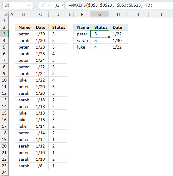
The MAXIFS and MINIFS functions were introduced in Excel 2016. Enter this formula as regular formula in cell G3:
Excel 2016 formula in cell H3:
These two formulas are entered as regular formulas.
3.1 Explaining the MAXIFS formula
The MAXIFS function calculates the highest value based on a condition or criteria.
Function syntax: MAXIFS(max_range, criteria_range1, criteria1, [criteria_range2, criteria2], ...)
MAXIFS(D3:D23, B3:B23, F3)
3.2 Explaining the MINIFS formula
The MINIFS function calculates the smallest value based on a given set of criteria.
Function syntax: MINIFS(min_range, criteria_range1, criteria1, [criteria_range2, criteria2], ...)
MINIFS(C3:C23, D3:D23, G3,B3:B23, F3)
4. Find and return the highest number and corresponding date based on a condition

This section describes how to filter records based on the maximum value of a specific item. There are names in column B, dates in column C, and numbers in column D. Use this formula if you are on an older Excel version than Excel 365.
The formula in cell G3 extracts numbers from column D based on the given condition in cell F3. The highest number is then calculated and returned to cell G3 with the corresponding date in column H.
Array formula in G3:
Array formula in cell H3:
4.1 How to enter an array formula
- Select cell F2.
- Paste formula in formula bar.
- Press and hold CTRL + SHIFT simultaneously.
- Press Enter once.
- Release all keys.
This is what the formula in the formula bar looks like:
Don't enter the curly brackets yourself, they appear automatically when you press CTRL + SHIFT + ENTER, see steps above.
Explaining array formula in cell G3
Step 1 - Find name in cell E2 in cell range B2:B22
The equal sign lets you compare a value to another value, you can also compare a value to an entire array of values. This is what we are going to do here.
The equal sign is one of many logical operators and the result is a boolean value TRUE or FALSE, or their numerical equivalents 1 (TRUE) or 0 (FALSE).
F3=$B$3:$B$23
becomes
"peter"={"peter"; "sarah"; "peter"; "sarah"; "peter"; "peter"; "sarah"; "luke"; "peter"; "sarah"; "sarah"; "peter"; "luke"; "luke"; "luke"; "peter"; "peter"; "sarah"; "peter"; "sarah"; "sarah"}
and returns
{TRUE; FALSE; TRUE; FALSE; TRUE; TRUE; FALSE; FALSE; TRUE; FALSE; FALSE; TRUE; FALSE; FALSE; FALSE; TRUE; TRUE; FALSE; TRUE; FALSE; FALSE}
Step 2 - Replace TRUE with corresponding value in cell range C2:C22 and FALSE with nothing
The IF function returns one value if the logical test is TRUE and another value if FALSE.
IF(logical_test, [value_if_true], [value_if_false])
IF(F3=$B$3:$B$23, $D$3:$D$23, "")
becomes
IF({TRUE; FALSE; TRUE; FALSE; TRUE; TRUE; FALSE; FALSE; TRUE; FALSE; FALSE; TRUE; FALSE; FALSE; FALSE; TRUE; TRUE; FALSE; TRUE; FALSE; FALSE}, $C$2:$C$22, "")
becomes
IF({TRUE; FALSE; TRUE; FALSE; TRUE; TRUE; FALSE; FALSE; TRUE; FALSE; FALSE; TRUE; FALSE; FALSE; FALSE; TRUE; TRUE; FALSE; TRUE; FALSE; FALSE}, {5; 5; 5; 4; 5; 5; 3; 4; 3; 3; 2; 2; 3; 3; 2; 2; 1; 2; 1; 2; 1}, "")
and returns
{5; ""; 5; ""; 5; 5; ""; ""; 3; ""; ""; 2; ""; ""; ""; 2; 1; ""; 1; ""; ""}
Step 3 - Find largest value in array
The MAX function returns the largest number froma cell range or an array.
MAX(IF(F3=$B$3:$B$23, $D$3:$D$23,""))
becomes
MAX({5; ""; 5; ""; 5; 5; ""; ""; 3; ""; ""; 2; ""; ""; ""; 2; 1; ""; 1; ""; ""})
and returns 5 in cell F2.
Explaining array formula in cell H3

Step 1 - Compare largest value with cell range $D$3:$D$23
This step returns an array containing boolean values, TRUE if they meet the condition and FALSE if not.
MAX(IF(F3=$B$3:$B$23, $D$3:$D$23, ""))=$D$3:$D$23
becomes
5=$D$3:$D$23
and returns
{TRUE; TRUE; TRUE; FALSE; TRUE; TRUE; FALSE; FALSE; FALSE; FALSE; FALSE; FALSE; FALSE; FALSE; FALSE; FALSE; FALSE; FALSE; FALSE; FALSE; FALSE}
Step 2 - Compare value in cell F3 with cell range $B$3:$B$23
This step compares the name in cell F3 to the values in cell range $B$3:$B$23.
F3=$B$3:$B$23
returns
{TRUE; FALSE; TRUE; FALSE; TRUE; TRUE; FALSE; FALSE; TRUE; FALSE; FALSE; TRUE; FALSE; FALSE; FALSE; TRUE; TRUE; FALSE; TRUE; FALSE; FALSE}
Step 3 - Multiply array in step 1 with array in step 2
This step applies AND logic meaning both conditions must be met in order to return TRUE.
TRUE * TRUE = TRUE (1)
TRUE * FALSE = FALSE (0)
FALSE * TRUE = FALSE (0)
FALSE * FALSE = FALSE (0)
When you multiply boolean values you always get the numerical equivalent, TRUE = 1 and FALSE = 0 (zero)
MIN(IF((MAX(IF(F3=$B$3:$B$23, $D$3:$D$23, ""))=$D$3:$D$23)*(F3=$B$3:$B$23),$C$3:$C$23, "A"))
MAX(IF(E2=$A$2:$A$22,$C$2:$C$22,""))=$C$2:$C$22)*(E2=$A$2:$A$22)
becomes
{TRUE; TRUE; TRUE; FALSE; TRUE; TRUE; FALSE; FALSE; FALSE; FALSE; FALSE; FALSE; FALSE; FALSE; FALSE; FALSE; FALSE; FALSE; FALSE; FALSE; FALSE} * {TRUE; FALSE; TRUE; FALSE; TRUE; TRUE; FALSE; FALSE; TRUE; FALSE; FALSE; TRUE; FALSE; FALSE; FALSE; TRUE; TRUE; FALSE; TRUE; FALSE; FALSE}
and returns
{1; 0; 1; 0; 1; 1; 0; 0; 0; 0; 0; 0; 0; 0; 0; 0; 0; 0; 0; 0; 0}
Step 4 - Replace TRUE with corresponding value in cell range C2:C22 and FALSE with random text string
The IF function returns one value if the logical test is TRUE and another value if FALSE.
IF(logical_test, [value_if_true], [value_if_false])
IF(E2=$A$2:$A$22,$C$2:$C$22,""))=$C$2:$C$22)*(E2=$A$2:$A$22),$B$2:$B$22,"A")
bcomes
IF({1; 0; 1; 0; 1; 1; 0; 0; 0; 0; 0; 0; 0; 0; 0; 0; 0; 0; 0; 0; 0},$B$2:$B$22,"A")
and returns
{42034; "A"; 42032; "A"; 42028; 42026; "A"; "A"; "A"; "A"; "A"; "A"; "A"; "A"; "A"; "A"; "A"; "A"; "A"; "A"; "A"}
Step 5 - Find smallest value in array, text strings are ignored
The MIN function returns the smallest number in a cell range or array, text strings are ignored.
MIN(IF((MAX(IF(E2=$A$2:$A$22,$C$2:$C$22,""))=$C$2:$C$22)*(E2=$A$2:$A$22),$B$2:$B$22,"A"))
becomes
MIN({42034; "A"; 42032; "A"; 42028; 42026; "A"; "A"; "A"; "A"; "A"; "A"; "A"; "A"; "A"; "A"; "A"; "A"; "A"; "A"; "A"})
and returns 42026 in cell G2.
5. Lookup value based on two critera - second criteria is the adjacent value and its position in a given list

This section demonstrates a formula that extracts items based on two conditions. The first condition (Location) is used to find a match in column B, the second condition is the adjacent value and its position in a list. The list (cell range G10:G13) looks like this:
- (blank)
- Low
- Medium
- High
If there are two matches (see image above, search value A matches two values) and the second condition is Low and Medium then the adjacent value to "Medium" is returned because it is further down in the list than "Low".
The formula returns values from cell range D3:D17 based on the position of the adjacent values in the above list. The image above shows that the condition in cell F3 matches the values in B14 and B16, however, the adjacent values in cell C14 and C16 determine which value to return. Cell C16 has a lower position in the list than cell C14. Value in cell D16 is returned.
This animated picture below shows you the most urgent work orders for a location. Type a location in cell F3 and the formula in cell G3 extracts the most urgent value for that particular location. The values in column C are 0 (blank), Low, Medium and High.
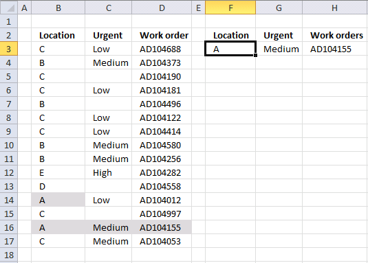
I have added conditional formatting to the table so you can quickly verify that the formulas in cell G3 and H3 are correct.
Formula in cell G3:
Formula in cell H3:
These formulas are array formulas if you own an Excel version previous to Excel 365 subscription.
How to enter an array formula
These steps are not required if you own an Excel 365 subscription.
- Copy above formula. Shortcut keys CTRL + c.
- Double-press with left mouse button on the destination cell.
- Paste formula to cell. Shortcut keys CTRL + v.
- Press and hold CTRL and SHIFT keys simultaneously.
- Press Enter once.
- Release all keys.
The formula bar changes, it now begins and ends with a curly bracket.

This tells you that the formula is an array formula.
5.1 Explaining the array formula in cell G3

It is much easier to understand and troubleshoot a formula if you use the "Evaluate Formula" tool. Select the cell containing a formula you want to examine.
Go to tab "Formulas" on the ribbon. Press with left mouse button on the "Evaluate Formula" button, a dialog box appears, see image above.
Press with left mouse button on the "Evaluate" button located on the dialog box to go through the calculations, step by step, in greater detail. The underlined expression is what is going to be evaluated next and the most recent evaluation is italicized.
Step 1 - Calculate the relative positions of values in column C with these values {0; "Low"; "Medium"; "High"}
The MATCH function returns the relative position of a given value in a cell range or array, however, in this demonstration, I will be using an array of values as lookup_value.
MATCH(lookup_value, lookup_array, [match_type])
The MATCH function is going to return an array of values that matches the number of values in the lookup_value.
MATCH($C$3:$C$17, {""; "Low"; "Medium"; "High"}, 0)
becomes
MATCH({"Low"; "Medium"; ""; "Low"; ""; "Low"; "Low"; "Medium"; "Medium"; "High"; ""; "Low"; ""; "Medium"; "Medium"}, {""; "Low"; "Medium"; "High"}, 0)
and returns the following array:
{2; 3; 1; 2; 1; 2; 2; 3; 3; 4; 1; 2; 1; 3; 3}
Step 2 - Extract values matching cell F3
The IF function checks which values in cell range B3:B17 that matches the search value in cell F3. If the logical expression returns TRUE the corresponding value is returned from the MATCH function calculation we did in step 1.
IF(F3=B3:B17, MATCH($C$3:$C$17, {0; "Low"; "Medium"; "High"}, 0), "")
becomes
IF(F3=B3:B17, {2; 3; 1; 2; 1; 2; 2; 3; 3; 4; 1; 2; 1; 3; 3} "")
becomes
IF("A"={"C"; "B"; "C"; "C"; "B"; "C"; "C"; "B"; "B"; "E"; "D"; "A"; "C"; "A"; "C"}, {2; 3; 1; 2; 1; 2; 2; 3; 3; 4; 1; 2; 1; 3; 3} "")
becomes
IF({FALSE; FALSE; FALSE; FALSE; FALSE; FALSE; FALSE; FALSE; FALSE; FALSE; FALSE; TRUE; FALSE; TRUE; FALSE}, {2; 3; 1; 2; 1; 2; 2; 3; 3; 4; 1; 2; 1; 3; 3} "")
and returns
{""; ""; ""; ""; ""; ""; ""; ""; ""; ""; ""; 2;""; 3;""}
Step 3 - Find the largest value
The MAX function returns the largest number from an array or cell range. It ignores text and blank values but not error values.
MAX(IF(F3=B3:B17, MATCH($C$3:$C$17, {0; "Low"; "Medium"; "High"}, 0), ""))
becomes
MAX({""; ""; ""; ""; ""; ""; ""; ""; ""; ""; ""; 2;""; 3;""})
and returns 3.
Step 4 - Return value
The INDEX function returns a value from a cell range or array based on a row and column number, the column number is optional if it is a one-dimensional cell range.
INDEX({""; "Low"; "Medium"; "High"}, MAX(IF(F3=B3:B17, MATCH($C$3:$C$17, {0; "Low"; "Medium"; "High"}, 0), "")))
becomes
INDEX({""; "Low"; "Medium"; "High"}, 3)
and returns "Medium" in cell G3.

The MATCH and MAX function returns the most urgent value in column C, the order of values in the array determines the importance. {0;"Low";"Medium","High"}. For example, "Medium" is more urgent than "Low". The MATCH function matches one set of values (column C) with another set of values {0;"Low";"Medium","High"}.
Explaining the array formula in cell H3
Step 1 - Evaluate logical test
The IF function returns a value based on what the logical_test returns, TRUE or FALSE. This step explains how the logical_test is calculated.
IF(logical_test, [value_if_true], [value_if_false])
The equal sign allows you to compare a cell to a cell range, the parentheses lets you control the order of operation.
($F$3=$B$3:$B$17)*($G$3=$C$3:$C$17)
becomes
("A"={"C"; "B"; "C"; "C"; "B"; "C"; "C"; "B"; "B"; "E"; "D"; "A"; "C"; "A"; "C"})*($G$3=$C$3:$C$17)
becomes
{FALSE; FALSE; FALSE; FALSE; FALSE; FALSE; FALSE; FALSE; FALSE; FALSE; FALSE; TRUE; FALSE; TRUE; FALSE}*($G$3=$C$3:$C$17)
becomes
{FALSE; FALSE; FALSE; FALSE; FALSE; FALSE; FALSE; FALSE; FALSE; FALSE; FALSE; TRUE; FALSE; TRUE; FALSE}*("Medium"={"Low";"Medium";0;"Low";0;"Low";"Low";"Medium";"Medium";"High";0;"Low";0;"Medium";"Medium"})
becomes
{FALSE; FALSE; FALSE; FALSE; FALSE; FALSE; FALSE; FALSE; FALSE; FALSE; FALSE; TRUE; FALSE; TRUE; FALSE}*{FALSE; TRUE; FALSE; FALSE; FALSE; FALSE; FALSE; TRUE; TRUE; FALSE; FALSE; FALSE; FALSE; TRUE; TRUE}
and returns
{0; 0; 0; 0; 0; 0; 0; 0; 0; 0; 0; 0; 0; 1; 0}
If you multiply a boolean value with a boolean value the result is always the numerical equivalent. TRUE -> 1 and FALSE -> 0 (zero)
Step 2 - Return corresponding values
The IF function replaces the array containing boolean values with values based on the outcome of the logical_test, TRUE (1) returns the second argument [value_if_true] and FALSE (0) returns the third argument [value_if_false].
IF(logical_test, [value_if_true], [value_if_false])
IF(($F$3=$B$3:$B$17)*($G$3=$C$3:$C$17), MATCH(ROW($B$3:$B$17), ROW($B$3:$B$17)), "")
The second argument contains these functions:
MATCH(ROW($B$3:$B$17), ROW($B$3:$B$17))
It creates an array containing a sequence from 1 to 15.
MATCH(ROW($B$3:$B$17), ROW($B$3:$B$17))
becomes
MATCH({3; 4; 5; 6; 7; 8; 9; 10; 11; 12; 13; 14; 15; 16; 17}, {3; 4; 5; 6; 7; 8; 9; 10; 11; 12; 13; 14; 15; 16; 17})
and returns
{1; 2; 3; 4; 5; 6; 7; 8; 9; 10; 11; 12; 13; 14; 15}
IF(($F$3=$B$3:$B$17)*($G$3=$C$3:$C$17), MATCH(ROW($B$3:$B$17), ROW($B$3:$B$17)), "")
becomes
IF({0; 0; 0; 0; 0; 0; 0; 0; 0; 0; 0; 0; 0; 1; 0}, MATCH(ROW($B$3:$B$17), ROW($B$3:$B$17)), "")
becomes
IF({0; 0; 0; 0; 0; 0; 0; 0; 0; 0; 0; 0; 0; 1; 0}, {1; 2; 3; 4; 5; 6; 7; 8; 9; 10; 11; 12; 13; 14; 15}, "")
and returns
{""; ""; ""; ""; ""; ""; ""; ""; ""; ""; ""; ""; ""; 14; ""}
Step 3 - Extract k-th smallest number
The SMALL function returns the k-th smallest number ina cell range or array. It ignores blanks and text values, however, not error values.
SMALL(array, k)
SMALL(IF(($F$3=$B$3:$B$17)*($G$3=$C$3:$C$17), MATCH(ROW($B$3:$B$17), ROW($B$3:$B$17)), ""), ROW(A1))
becomes
SMALL({""; ""; ""; ""; ""; ""; ""; ""; ""; ""; ""; ""; ""; 14; ""}, ROW(A1))
becomes
SMALL({""; ""; ""; ""; ""; ""; ""; ""; ""; ""; ""; ""; ""; 14; ""}, 1)
and returns 14.
Step 4 - Return value
The INDEX function returns a value from a table based on row and column number. The column number is optional if you only fetch values from a single column.
INDEX(array, [row_num], [column_num])
INDEX($D$3:$D$17, SMALL(IF(($F$3=$B$3:$B$17)*($G$3=$C$3:$C$17), MATCH(ROW($B$3:$B$17), ROW($B$3:$B$17)), ""),ROW(A1)))
becomes
INDEX($D$3:$D$17, 14)
and returns "AD104155" in cell H3.
Step 5 - Catch error
The IFERROR function traps errors and allows you to return any value if an error has occurred. The IFERROR function returns a blank cell if an error is returned.
Be careful with the IFERROR function, it can make it very difficult to find errors in a worksheet.
IFERROR(value, value_if_error)
IFERROR(INDEX($D$3:$D$17, SMALL(IF(($F$3=$B$3:$B$17)*($G$3=$C$3:$C$17), MATCH(ROW($B$3:$B$17), ROW($B$3:$B$17)), ""),ROW(A1))), "")
More than 1300 Excel formulasExcel categories
One Response to “Find and return the highest number and corresponding date based on a condition”
Leave a Reply
How to comment
How to add a formula to your comment
<code>Insert your formula here.</code>
Convert less than and larger than signs
Use html character entities instead of less than and larger than signs.
< becomes < and > becomes >
How to add VBA code to your comment
[vb 1="vbnet" language=","]
Put your VBA code here.
[/vb]
How to add a picture to your comment:
Upload picture to postimage.org or imgur
Paste image link to your comment.
Just because I've noticed this
"Step 2 - Compare value in cell E2 with cell range A2:A2"
you miss the last 2 on A22 range
thanks for all your advice, I discover your site today and I felt in love