Split data across multiple sheets – VBA
Table of Contents
- Split data across multiple sheets - VBA
- Add values to worksheets based on a condition - VBA
- Basic data entry - VBA
- Add values to a two-dimensional table based on conditions - VBA
- Split values equally into groups
- Rearrange values based on category - VBA
- How to group items by quarter using formulas
- Automate data entry - VBA
1. Split data across multiple sheets - VBA
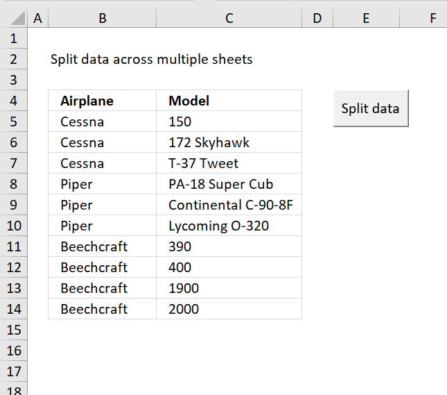
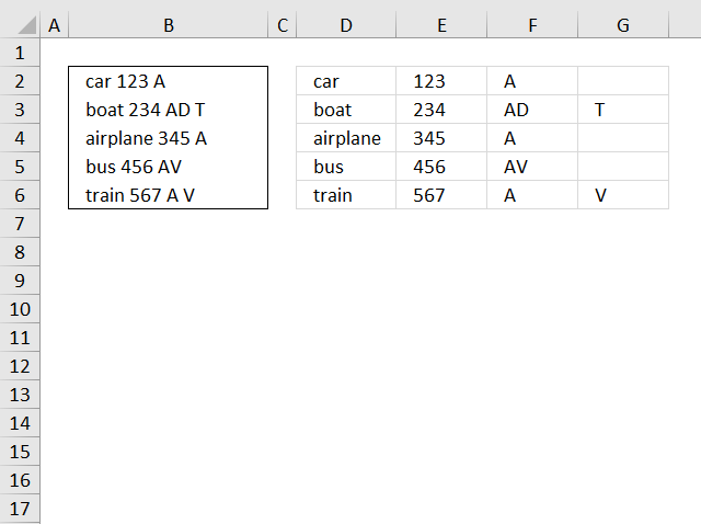
In this section I am going to show how to create a new sheet for each airplane using vba. The macro copies airplane and model values into each new sheet.
Before:

After:

The Code
Sub Splitdatatosheets()

' Splitdatatosheets Macro
Dim rng As Range
Dim rng1 As Range
Dim vrb As Boolean
Dim sht As Worksheet
Set rng = Sheets("Sheet1").Range("A4")
Set rng1 = Sheets("Sheet1").Range("A4:D4")
vrb = False
Do While rng <> ""
For Each sht In Worksheets
If sht.Name = Left(rng.Value, 31) Then
sht.Select
Range("A2").Select
Do While Selection <> ""
ActiveCell.Offset(1, 0).Activate
Loop
rng1.Copy ActiveCell
ActiveCell.Offset(1, 0).Activate
Set rng1 = rng1.Offset(1, 0)
Set rng = rng.Offset(1, 0)
vrb = True
End If
Next sht
If vrb = False Then
Sheets.Add After:=Sheets(Sheets.Count)
ActiveSheet.Name = Left(rng.Value, 31)
Sheets("Sheet1").Range("A3:B3").Copy ActiveSheet.Range("A1")
Range("A2").Select
Do While Selection <> ""
ActiveCell.Offset(1, 0).Activate
Loop
rng1.Copy ActiveCell
Set rng1 = rng1.Offset(1, 0)
Set rng = rng.Offset(1, 0)
End If
vrb = False
Loop
End Sub
Get excel tutorial file
Remember to enable macros and backup your excel file because you can´t undo macros.
Split-data-across-multiple-sheets.xls
(Excel 97-2003 Workbook *.xls)
Split Data Across Multiple Sheets Add-In
Split data across multiple sheets Add-In for Excel let´s you split/categorize data from a sheet across multiple new sheets.

Features
- Select any single range
- Select specific columns
- Arrange output columns in any order
- Categorize data across sheets in current workbook, new workbook or any open workbook
- Add column headers to each new sheet
What you get
- Split data across multiple sheets add-in for Excel *.xlam file.
- Instructions on how to install.
- Instructions on how to use.
- Excel *.xlsx example file.
- 2 licenses, home and office computer.
Questions:
Is there a money back guarantee?
Sure, you have unconditional money back guarantee for 14 days.
What about working with merged cells?
The add-in won't work with merged cells. Unmerge cells before usage.
I have more questions?
Use this contact form to let me know.
Purchase Split Data Across Multiple Sheets Add-In for Excel - Price $19 US


2. Add values to worksheets based on a condition - VBA
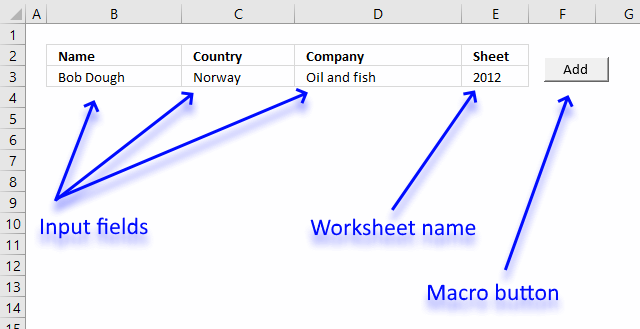
This tutorial shows you how to add a record to a particular worksheet based on a condition, the image above shows input fields name, country, company and sheet.
The sheet input field determines which worksheet to add the values to, the add button allows you to run the macro and place the values automatically.
I will also show you the macro code to accomplish this task, what each line does, and where to put the code.
This section is inspired by this question:

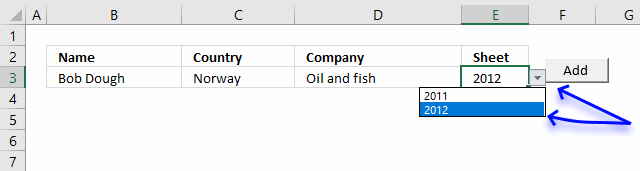
The animated image above demonstrates how to type input values and then cut values and paste to the given worksheet.
To make things easier a drop down list lets the user pick worksheet name in cell D2.
How to create a drop down list
- Select cell E2.
- Go to tab "Data" on the ribbon.
- Press with left mouse button on "Data Validation" button.
- Go to "Settings" tab.
- Select List
- Type 2011, 2012 (sheet names) in Source:
- Press with left mouse button on OK
A black arrow appears next to cell E2, see image above. Press with left mouse button on the arrow to expand a list that allows you to select a worksheet name.
Where to put the code?
- Copy code below.
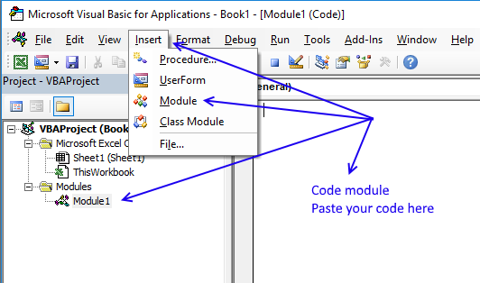
- Go to Excel and press Alt+ F11 to open the VB Editor (Visual Basic Editor).
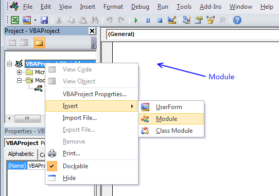
- Select your workbook in the Project Explorer.
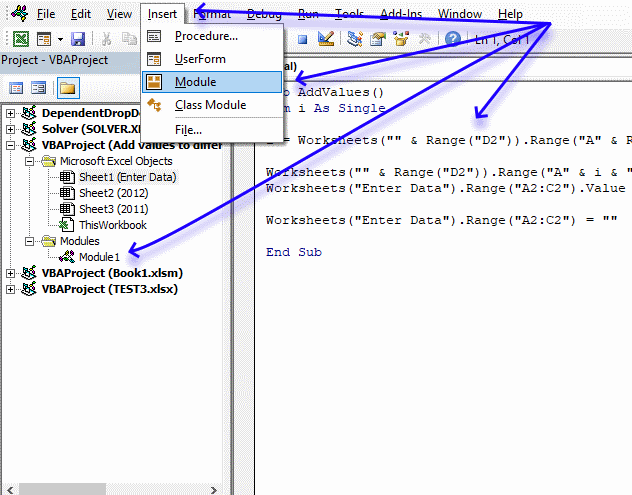
- Press with left mouse button on Insert on the menu.
- Press with left mouse button on Module to insert a module to the selected workbook.
- Paste macro code to the code module.
- Exit VB Editor.
VBA code
'Name macro
Sub AddValues()

'Dimension variable and declare data type
Dim i As Single

'Save row number of cell below last nonempty cell
i = Worksheets("" & Range("E3")).Range("A" & Rows.Count).End(xlUp).Row + 1

'Save input values to selected worksheet
Worksheets("" & Range("E3")).Range("A" & i & ":C" & i) = _
Worksheets("Enter Data").Range("B3:D3").Value

'Clear input cells
Worksheets("Enter Data").Range("A2:C2") = ""

'Stop macro
End Sub
Create a press with left mouse button onable button that runs a macro
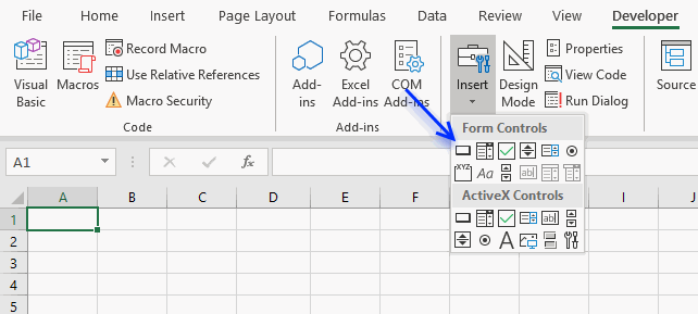
- Go to "Developer" tab on the ribbon.
- Press with left mouse button on "Insert" button.
- Press with left mouse button on "Button" (Form Control).
- Press with left mouse button on and drag on worksheet to create button.
- Assign macro AddValues
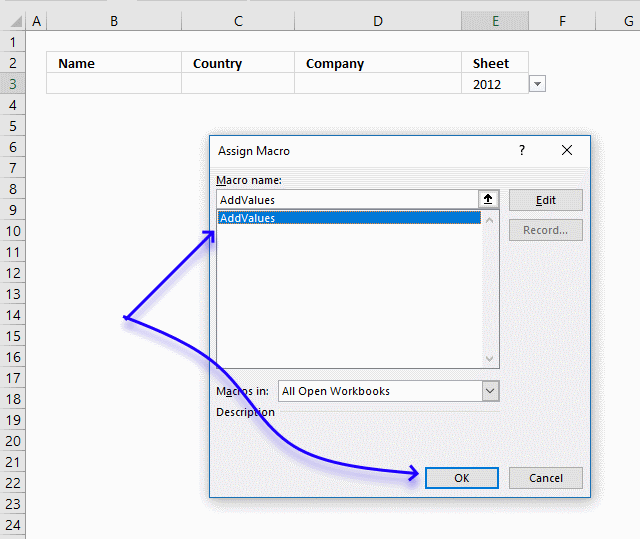
- Press with left mouse button on OK button.
Press with left mouse button on the button to run macro AddValues.
3. Basic data entry - VBA

In this small tutorial, I am going to show you how to create basic data entry with a small amount of VBA code.
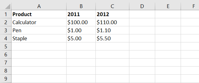
Cell B3 and C3 are input cells. When you press with left mouse button on button "Add", the data in cell B3 and C3 are copied to the first empty row in the list.
The last step in the code removes the values in cell B3 and C3, see the animated image above.
3.1. Data entry - VBA Macro
'Name macro
Sub AddText()

'Dimension variables and declare data types
Dim Lrow As Single

With Worksheets("Sheet1")
'Find last non-empty cell in column B
Lrow = .Range("B" & Rows.Count).End(xlUp).Row + 1

'Copy values
.Range("B" & Lrow & ":C" & Lrow) = .Range("B3:C3").Value

'Delete values
.Range("B3:C3").Value = ""
End With

End Sub
3.2. How to insert the VBA macro to your workbook
- Press Alt+F11 to open the VB Editor.
- Press with right mouse button on on your workbook name in the Project Explorer window.
- Press with left mouse button on "Insert".
- Press with left mouse button on "Module" to insert a code module to your workbook.
- Copy macro and paste to code module, see image above.
3.4. Simplify VBA code further
Worksheets("Sheet1") is repeated many times. The WITH and WITH END statement allows you to simplify the code.
Sub AddText()
Dim Lrow As Single
With Worksheets("Sheet1")
Lrow = .Range("B" & Rows.Count).End(xlUp).Row + 1
.Range("B" & Lrow & ":C" & Lrow) = .Range("B3:C3").Value
.Range("B3:C3").Value = ""
End With
End Sub
3.5. How to insert a button
- Go to the Developer tab.
- Press with left mouse button on "Insert" button on the ribbon.
- Press with left mouse button on "Button" (Form Control).
- Press and hold with left mouse button on the worksheet.
- Drag with mouse to create the button then release the mouse button.
3.6. How to assign a macro to a button
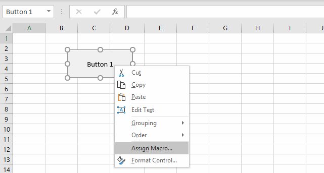
- Press with right mouse button on on your new button.
- Assign a macro.
- Select "AddText" macro.
Final note
There is a data entry form in Excel but it is not on the ribbon.
4. Add values to a two-dimensional table based on conditions - VBA
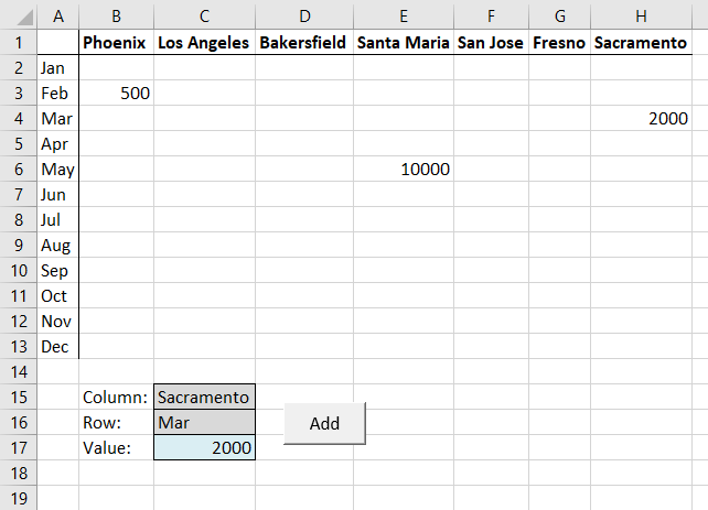
This article demonstrates how to place values automatically to a table based on two conditions using a short macro.
Cell C15 and C16 contain the conditions, they both allow you to select a value using drop down lists. Cell C17 contains the value you want to place, type this value and then press Enter.
The example shown above is based on the question below:
I do remember seeing one nice way of populating a table with the use of vba such as :
Sub EnterName()

Dim col As Single, Lrow As Single
Dim tmp As String

col = Application.WorksheetFunction.Match(Range("C2"), Range("B4:H4"), 0) - 1
tmp = Range("B" & Rows.Count).Offset(0, col).Address
Lrow = Range(tmp).End(xlUp).Row

Range("B1").Offset(Lrow, col).Value = Range("E2").Value
Range("B1").Offset(Lrow, col + 1).Value = Range("F2").Value
Range("E2").Value = ""
Range("F2").Value = ""

End Sub
How would it be possible to modify the code to populate a table such as: the first column header could be chosen from the drop-down list as well as the first row header. In other word the location of the data to be entered could be determined by the row AND the column.
C2 should be a data validation (list).
B4:H4 (here only 7 columns) would be the headers to match the value in C2.
A second data validation should make reference to Column A.
Hence:
1st data validation correlated to Column's Headers (B to ect)
2nd data validation correlated to values in Column A ("Row Header")
As for the kind of values, being headers they would most likely be (but not limited to) text strings.

The animated image above demonstrates how it works, simply pick values in the drop down lists, enter a value in C17 and then press on the button containing text value "Add".
4.1 Create drop down lists
- Select cell C15
- Go to tab "Data"
- Press with left mouse button on "Data validation" button
- Select "List" in Allow: field
- Select cell range B1:H1 in Source: field
Repeat above steps with cell C16 and cell range A2:A13
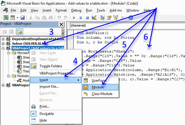
4.2 How to add macro to your workbook
- Copy VBA code below.
- Press Alt+ F11 to open the VBE (Visual Basic Editor).
- Press with right mouse button on on your workbook in project explorer to open a context menu.
- Press with left mouse button on Insert on the menu.
- Press with left mouse button on Module on the menu.
- Paste VBA code to module window.
- Return to Excel
4.3 VBA macro
'Name macro
Sub AddValue()

'Dimension variables and declare data types
Dim column as String, row As String
Dim c As Single, r As Single

'The With - End With allows you write shorter lines of code by referring to an object only once instead of using it with each property.
With Worksheets("Sheet1")

'Stop macro if cell C15 or C16 is empty
If .Range("C15").Value = "" Or .Range("C16").Value = "" Then Exit Sub

'Save value in cell C15 to variable column
column = .Range("C15").Value

Save value in cell C16 to variable row
row = .Range("C16").Value

'Find relative position of value in cell C15 in cell range B1:H1 and save to variable c
c = Application.Match(column, .Range("B1:H1"), 0)

'Find relative position of value in cell C16 in cell range A2:A13 and save to variable r
r = Application.Match(row, .Range("A2:A13"), 0)

'Save value to table using coordinates
.Range("A1").Offset(r, c).Value = .Range("C17").Value

End With

'Stop macro
End Sub
4.4 How to create a press with left mouse button onable button on worksheet and link it to a macro
- Go to "Developer" tab on the ribbon.
- Press with left mouse button on "Insert" button.
- Press with left mouse button on "Button".
- Press with left mouse button on and drag on worksheet to create a button.
- Press with right mouse button on on macro to display a context menu, press with left mouse button on "Assign macro".
- Select macro "Add Value".
- Press with left mouse button on OK
- Press with mouse on button text to show prompt, then change button text to "Add".
5. Split values equally into groups
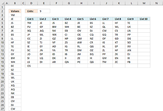
This post shows you two different approaches, an array formula, and a User Defined Function. You will find the UDF later in this post.
The above picture shows you values in column A and they are equally split across 9 columns, column D to M.
Formula in D5:
Now copy cell D5 and paste to cells below and to the right.
5.1 Explaining formula in cell D5
Step - 1 Keep track of lists
The COLUMNS function works just like the ROWS function except it counts columns instead of rows in a cell reference.
| Cell | COLUMNS function | Result |
| D5 | COLUMNS($A$1:A1) | 1 |
| E5 | COLUMNS($A$1:A2) | 2 |
| F5 | COLUMNS($A$1:A3) | 3 |
Cell E2 contains the number of lists to put the values into.
$E$2>=COLUMNS($A$1:A1) returns TRUE. This makes the formula return blank cells when the number of lists are greater than the value in cell E2.
Step 2 - Return blanks if all lists are populated
The IF function lets you specify a value if the logical expression returns TRUE (argument 2) and another value if FALSE (argument 3).
IF($E$2>=COLUMNS($A$1:A1),INDEX($B$3:$B$102,(ROWS($A$1:A1))*$E$2-($E$2-COLUMNS($A$1:A1))),"")
returns INDEX($B$3:$B$102,(ROWS($A$1:A1))*$E$2-($E$2-COLUMNS($A$1:A1)))
Step 3 - Return number based on an expanding cell reference
The ROWS function returns the number of rows in a cell reference, this cell ref is special. It expands as the formula is copied to cells below.
ROWS($A$1:A1)
returns 1.
| Cell | ROWS function | Result |
| B3 | ROWS($A$1:A1) | 1 |
| B4 | ROWS($A$1:A2) | 2 |
| B5 | ROWS($A$1:A3) | 3 |
Step 4 - Multiply with cell E2
ROWS($A$1:A1)*$E$2 becomes 1*9 equals 9.
Step 5 - Subtract $E$2 with COLUMNS
$E$2-COLUMNS($A$1:A1)) becomes 9-1 equals 8
Step 6 - Calculate row number
ROWS($A$1:A1)*$E$2-($E$2-COLUMNS($A$1:A1)) becomes 9-8 equals 1.
Step 6 - Get value based on row number
The INDEX function returns a value in cell range based on a row and column number. This is a single column cell ref so the column number is not neccessary in this case.
INDEX($B$3:$B$102,(ROWS($A$1:A1))*$E$2-($E$2-COLUMNS($A$1:A1))) returns "YM" in cell D5.
5.2 User defined function
You decide how many groups you want by selecting a cell range with as many columns as you want groups and then enter the UDF. It is designed to group values depending on how many columns you have selected before entering it.
The animated picture above shows you a cell range with 5 columns.
5.3 How to enter an array formula
- Select cell range C2:G11
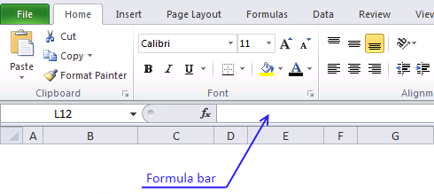
- Paste above array formula to your formula bar
- Press and hold CTRL and SHIFT keys simultaneously
- Press Enter once
The formula in the formula bar now looks like this: {=GroupValues(A2:A24)}
Don't enter these curly parentheses yourself, they appear automatically if you did the above steps correctly.
Recommended articles

Array formulas allows you to do advanced calculations not possible with regular formulas.
5.4 VBA code
Function GroupValues(rng As Range)
Dim result As Variant
c = Application.Caller.Columns.Count
r = Application.Caller.Rows.Count
ReDim result(1 To r, 1 To c)
i = 1
For ro = 1 To r
    For co = 1 To c
        If rng.Cells(i) <> "" Then
            result(ro, co) = rng.Cells(i)
        Else
            result(ro, co) = ""
        End If
        i = i + 1
    Next co
Next ro
GroupValues = result
End Function
5.5 How do I copy the code to my workbook?
- Open VB editor (Alt+F11)
- Insert a module to your workbook
- Paste code to code module
- Go back to Excel
6. Rearrange values based on category - VBA
In this post I am going to rearrange values from a list into unique columns.
Before:

After:

6.1 The code
Sub Categorizedatatocolumns()

Dim rng As Range

Dim dest As Range

Dim vrb As Boolean

Dim i As Integer

Set rng = Sheets("Sheet1").Range("A4")

vrb = False

Do While rng <> ""

Set dest = Sheets("Sheet1").Range("A20")

Do While dest <> ""

If rng.Value = dest.Value Then

vrb = True

End If

Set dest = dest.Offset(0, 1)

Loop

If vrb = False Then

dest.Value = rng.Value

dest.Font.bold = True

End If

vrb = False

Set rng = rng.Offset(1, 0)

Loop

Set rng = Sheets("Sheet1").Range("A4")

Do While rng <> ""

Set dest = Sheets("Sheet1").Range("A20")

Do While dest <> ""

If rng.Value = dest.Value Then

i = 0

Do While dest <> ""

Set dest = dest.Offset(1, 0)

i = i + 1

Loop

Set rng = rng.Offset(0, 1)

dest.Value = rng.Value

Set rng = rng.Offset(0, -1)

Set dest = dest.Offset(-i, 0)

End If

Set dest = dest.Offset(0, 1)

Loop

Set rng = rng.Offset(1, 0)

Loop

End Sub
Get Excel file
Remember to backup your excel workbook, you can't undo macros.
Categorize-data-into-multiple-columns.xls
(Excel 97-2003 Workbook *.xls)
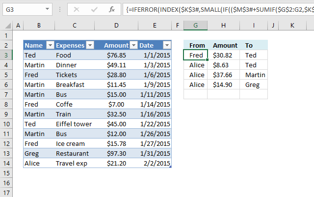
7. How to group items by quarter using formulas
This article demonstrates two formulas, the first formula counts items by quarter and the second formula extracts the corresponding items horizontally.
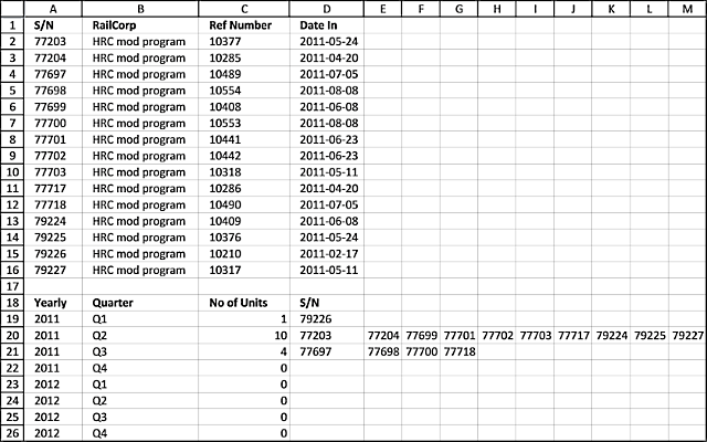
The image above shows a formula in cell C19 that extracts numbers from column A based on the corresponding date in column D. If the date is in a given year and quarter specified in cell A19 and B19 and cells below the numbers show up in column E and columns to the right as far as needed.
77203 HRC mod program 10377 24/05/2011
77204 HRC mod program 10285 20/04/2011
77697 HRC mod program 10489 5/07/2011
77698 HRC mod program 10554 8/08/2011
77699 HRC mod program 10408 8/06/2011
77700 HRC mod program 10553 8/08/2011
77701 HRC mod program 10441 23/06/2011
77702 HRC mod program 10442 23/06/2011
77703 HRC mod program 10318 11/05/2011
77717 HRC mod program 10286 20/04/2011
77718 HRC mod program 10490 5/07/2011
79224 HRC mod program 10409 8/06/2011
79225 HRC mod program 10376 24/05/2011
79226 HRC mod program 10210 17/02/2011
79227 HRC mod program 10317 11/05/2011
I don't want to input the S/N in Table 2 manually. I need a formula for it as this is only part of the data that I need to categorize.I need the S/N listed by the quarter they came in (Date In).Yearly Quarter No Of Units S/NQ1-2011 1
Q2-2011 10
Q3-2011 4
Q4-2011 0
Q1-2012 0
If someone can please help.this is the result I am after but it should be done using formulasYearly Quarter No Of Units S/NQ1-2011 1 79226
Q2-2011 10 77203, 77204, 77699, 77701, 77702, 77703, 77717, 79224, 79225, 79227
Q3-2011 4 77697, 77698, 77700, 77718
Q4-2011 0 NA
Q1-2012 0 NA
Thanks in Advance
Answer:
Formula in cell C19:
Array formula in cell D19:
How to enter an array formula
- Double press with left mouse button on cell D19
- Copy above formula and paste to cell D19
- Press and hold CTRL + SHIFT simultaneously.
- Press Enter once.
If you did it right the formula now has curly brackets before and after the formula, like this ={formula}. Don't enter these characters yourself.
Explaining formula in cell C19

I recommend the "Evaluate Formula" tool if you want to understand formulas in greater detail. They let you check each calculation step, simply press with left mouse button on the "Evaluate" button to move to the next calculation step.
Here is how to start it. Select the cell containing a formula you want to check out. Press with left mouse button on "Formulas" on the ribbon and the press with left mouse button on "Evaluate Formulas" tool.
This opens the "Evaluate Formula" dialog box. The evaluation window is populated with the formula of the selected cell.
The underlined expression is what is next to be evaluated and the italicized text is the last evaluation. This allows you to follow the calculations in detail, simply press with left mouse button on the "Evaluate" button to move to the next calculation until the final result is displayed. Press with left mouse button on the "Close" button to dismiss the dialog box.
Step 1 - Calculate start month
The RIGHT function takes the first character from the right. Q1 becomes 1.
RIGHT(B19,1)
becomes
RIGHT("Q1",1)
and returns "1".
The CHOOSE function allows you to get a value based on a number. The number represents the position of the returned value.
CHOOSE(RIGHT(B19,1), 1,4,7,10)
becomes
CHOOSE(1, 1,4,7,10)
and returns 1.
Step 2 - Create the start date
The DATE function creates an Excel date based on a year, month, and day value.
DATE(A19, CHOOSE(RIGHT(B19,1), 1,4,7,10), 1)
becomes
DATE(2011, 1, 1)
and returns 2011-01-01
Step 3- Calculate the end date
DATE($A19, CHOOSE(RIGHT($B19,1), 4,7,10,1), 1)-1
becomes
DATE($A19, 4, 1)-1
becomes
(2011-04-01)-1
returns 2011-03-31.
Step 4 - Count records in the date range
The COUNTIFS function allows you to use multiple conditions. Dates larger than or equal to the start date and dates smaller than or equal to the end date.
COUNTIFS($D$2:$D$16, ">="&DATE(A19, CHOOSE(RIGHT(B19,1), 1,4,7,10), 1), $D$2:$D$16, "<="&DATE(A19, CHOOSE(RIGHT(B19,1), 4,7,10,1), 1)-1)
becomes
COUNTIFS($D$2:$D$16, ">="&2011-01-01, $D$2:$D$16, "<="&"2011-03-31")
and returns 1.
Explaining formula in cell D19
Step 1 - Find out which values are in a quarter and return their row number
I am not going to explain how to calculate the date ranges again, see steps 1 - 3 above.
The IF function returns one value if the logical test is TRUE and another value if the logical test is FALSE. IF(logical_test, [value_if_true], [value_if_false])
In this case, the IF function extracts numbers of those rows that have a date in the date range.
IF(($D$2:$D$16>=(DATE($A19, CHOOSE(RIGHT($B19,1), 1,4,7,10), 1)))*($D$2:$D$16<=(DATE($A19, CHOOSE(RIGHT($B19,1), 4,7,10,1), 1)-1)), MATCH(ROW($D$2:$D$16), ROW($D$2:$D$16)), "")
becomes
IF(($D$2:$D$16>="2011-01-01")*($D$2:$D$16<="2011-03-31", MATCH(ROW($D$2:$D$16), ROW($D$2:$D$16)), "")
becomes
IF(({FALSE; FALSE; FALSE; FALSE; FALSE; FALSE; FALSE;FALSE; FALSE;FALSE; TRUE;FALSE; FALSE;FALSE; FALSE})*({TRUE; TRUE;TRUE;TRUE; TRUE;TRUE; TRUE;TRUE; TRUE;TRUE; TRUE;TRUE; TRUE;TRUE; TRUE}), MATCH(ROW($D$2:$D$16), ROW($D$2:$D$16)), "")
becomes
IF({0; 0; 0; 0; 0; 0; 0; 0; 0; 0; 0; 0; 0; 1; 0}, MATCH(ROW($D$2:$D$16), ROW($D$2:$D$16)), "")
The ROW and MATCH functions creates a sequence from 1 to n where n is the number of rows in cell range $D$2:$D$16. These row numbers allow you to extract the corresponding values from cell range A2:A16 in a later step.
and returns {"";"";"";"";"";"";"";"";"";"";"";"";"";14;""}
Step 2 - Extract row number
SMALL(IF(($D$2:$D$16>=(DATE($A19, CHOOSE(RIGHT($B19, 1), 1, 4, 7, 10), 1)))*($D$2:$D$16<=(DATE($A19, CHOOSE(RIGHT($B19, 1), 4, 7, 10, 1), 1)-1)), MATCH(ROW($D$2:$D$16), ROW($D$2:$D$16)), ""), COLUMN(A1))
becomes
SMALL({"";"";"";"";"";"";"";"";"";"";"";"";"";14;""}, COLUMN(A1)) and returns 14.
Step 3 - Return value
INDEX($A$2:$A$16, SMALL(IF(($D$2:$D$16>=(DATE($A19, CHOOSE(RIGHT($B19,1), 1,4,7,10), 1)))*($D$2:$D$16<=(DATE($A19, CHOOSE(RIGHT($B19,1), 4,7,10,1), 1)-1)), MATCH(ROW($D$2:$D$16), ROW($D$2:$D$16)), ""),COLUMN(A1)))
becomes
INDEX($A$2:$A$16, 14)
becomes
INDEX({77203; 77204; 77697; 77698; 77699; 77700; 77701; 77702; 77703; 77717; 77718; 79224; 79225; 79226; 79227}, 14)
and returns 79226 in cell D19.
8. Automate data entry - VBA
This article demonstrates how to automatically enter data in cells if an adjacent cell is populated using VBA code.
In some cases, it can be useful and timesaving to automate data entering, the VBA examples here all enter a value or formula in a cell if a value is entered by the user in the adjacent column.
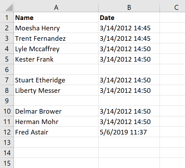
The image above shows a worksheet that enters a timestamp in column B if the corresponding cell in column A is populated.
VBA enters timestamp automatically in the adjacent cell
Enter a name in column A and current date and time is entered automatically in column B. You can also copy a cell range and paste them to column A. Empty cells are not processed.
What makes this work is an event code that catches changes on a worksheet, this makes it possible to populate the adjacent cell with whatever you want. I am in this case entering a time stamp in column B.

VBA code
'Event procedure that is rund if any cell on the worksheet is changed
Private Sub Worksheet_Change(ByVal Target As Range)

'Dimension variable and data type
Dim Value As Variant

'If target cell (the cell that changed) is in column A then do this.
If Not Intersect(Target, Range("A:A")) Is Nothing Then

    'Repeat these lines as many times as there were cells that changed
    For Each Value In Target

        'If value is not equalt to nothing then do this.
        If Value <> "" Then

            'Populate adjacent cell in column B based on row number from target cell
            Range("B" & Value.Row).Value = Now
        End If
    Next Value
End If
End Sub
Where to copy code?
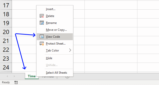
- Press with right mouse button on on the sheet name
- Press with left mouse button on "View code" to open the VB Editor.
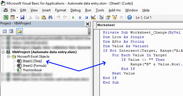
- Copy/Paste vba code to sheet module, see image above.
Populate a cell with a formula using VBA

The following VBA code populates the adjacent cell in column C with a formula if corresponding cell value in column B is populated.
Here is what I did: Enter a price in column B and a formula is instantly entered in column C. Formula in column c: Cell value in column B multiplied by 1.1
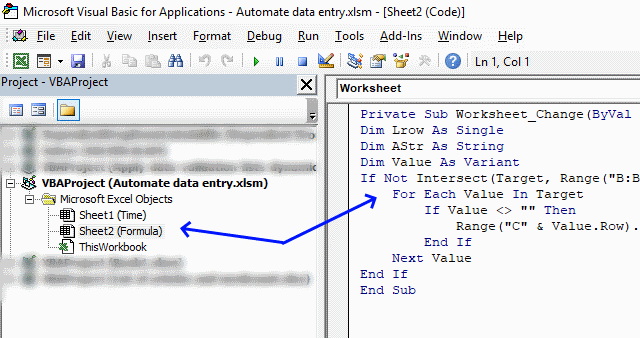
VBA code
'Event code that runs if a cell or cell range is changed
Private Sub Worksheet_Change(ByVal Target As Range)

'Dimension variables and declare data types
Dim Lrow As Single
Dim AStr As String
Dim Value As Variant

'Check if cell or cell range that changed is in column B
If Not Intersect(Target, Range("B:B")) Is Nothing Then

    'Repeat the following code as many times as there a cells in the cell range that changed
    For Each Value In Target

        'Check if cell (that changed) is not equal to nothing
        If Value <> "" Then

            'Populate adjacent cell in column C with a formula
            Range("C" & Value.Row).Formula = "=" & Target.Address & "*1.1"
        End If
    Next Value
End If
End Sub
Where to copy code?
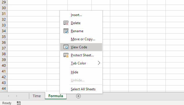
- Press with right mouse button on on current sheet name
- Press with left mouse button on "View code"
- Copy/Paste vba code to sheet module.
- Copy/Paste vba code to sheet module, see image above.
Final notes
The techniques demonstrated here in this article should give you a great start in automating data entry in your workbook.
Keep in mind that if you happen to get caught in an endless loop because the code changes a value that then triggers the event code over and over you can prevent this by using the Application.EnableEvents property.
Application.EnableEvents = False

Code

Application.EnableEvents = True
This will stop the event code from triggering while the macro manipulates the worksheet.
The first example above automatically enters the timestamp, however, if want to know how to manually enter a timestamp then use following shortcut keys: CTRL + :
The second example can be done using formulas as well, you can also use a formula that will output nothing if the adjacent value is empty.
Formula in cell C2:
This formula will check if cell B2 is not empty and then multiply that value with 1.1 if TRUE and return a blank if FALSE.
B2<>"" is a logical expression that returns either TRUE or FALSE. If B2 is not empty the logical expression returns TRUE and if it is empty the logical expression returns FALSE.
IF(logical_expression, if_true, if_false)
The IF function then runs the second argument if the logical expression returns TRUE and the third argument if FALSE.
You can read more about this function here: IF function
Add in category
Macro category
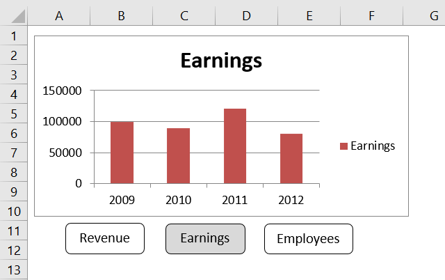
Table of Contents How to create an interactive Excel chart How to filter chart data How to build an interactive […]
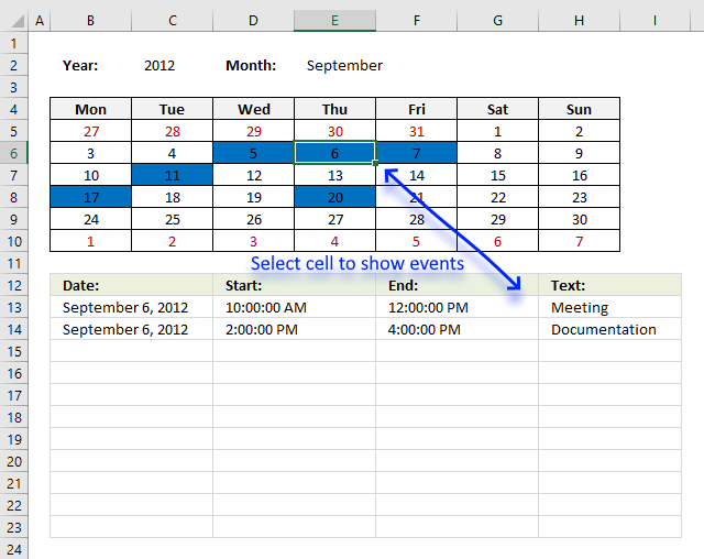
Table of Contents Excel monthly calendar - VBA Calendar Drop down lists Headers Calculating dates (formula) Conditional formatting Today Dates […]
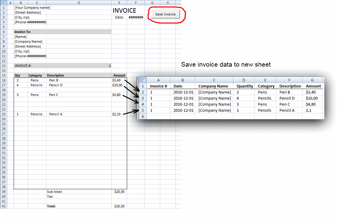
Table of contents Save invoice data - VBA Invoice template with dependent drop down lists Select and view invoice - […]
Split values category
This blog article describes how to split strings in a cell with space as a delimiting character, like Text to […]
This article demonstrates two ways to calculate expenses evenly split across multiple people. The first one is a formula solution, […]
Excel categories
68 Responses to “Split data across multiple sheets – VBA”
Leave a Reply
How to comment
How to add a formula to your comment
<code>Insert your formula here.</code>
Convert less than and larger than signs
Use html character entities instead of less than and larger than signs.
< becomes < and > becomes >
How to add VBA code to your comment
[vb 1="vbnet" language=","]
Put your VBA code here.
[/vb]
How to add a picture to your comment:
Upload picture to postimage.org or imgur
Paste image link to your comment.
how would we print the sorted sheet into a new workbook rather than the same?
how do we set a range on the column. Say you only wanted to split the information between a4 and a10 rather than between a4 and the very end of the list.
Great - worked a charm.
“Split data across multiple sheets in excel (vba)”...
this code works well, but the prob is could not able to get the Merge cell as it is..
Thnx
Mashini,
I don´t have an answer right now.
I found this:
Excel often has problems copying ranges containing merged cells onto sheets with merged cells even if the merged areas are the same. The best solution is to not have merged cells. Next best is to unmerge all cells in the range that is to receive the copy before pasting in the new data.
from here
Hej.. works...problem is for a huge file.. doesn't. I have a 470k rows and is blocking at some point.
Alin,
Where does it halt and what does the row look like? You can use this contact form.
Awesome....
Thanks!
thnak you very much, its really helpful for me
It is really a nice article. I have used it in one of my automation but it goes into loop and never ends. I have to abruptly log off from the system to stop it. Need urgent help on it.
sujay,
can you provide an example of your sheet?
Hi,
I am new to Excel with VBA code.. I have 1 excel with 2 sheets ( A.xl contains 2 tabs Name and Rating ).
I want to read the datas from 2 sheets (Name and Rating) and appened the data in other excel file..
Can any one please help me to solve this...
Hi there!
This code is working perfectly for me besides the fact that the macro stops splitting my table into different sheets once it reaches a field name longer that 31 characters. Is there any way I can work around this?
Nice work...
Jojo,
Yes, I have uploaded a new file and changed the post.
Thanks for commenting!
Peter,
Thanks!
Lovely! Thanks so much Oscar.
Oscar,
I do remember seeing one nice way of populating a table with the use of vba such as :
Sub EnterName()
Dim col, Lrow As Single
Dim tmp As String
col = Application.WorksheetFunction.Match(Range("C2"), Range("B4:H4"), 0) - 1
tmp = Range("B" & Rows.Count).Offset(0, col).Address
Lrow = Range(tmp).End(xlUp).Row
Range("B1").Offset(Lrow, col).Value = Range("E2").Value
Range("B1").Offset(Lrow, col + 1).Value = Range("F2").Value
Range("E2").Value = ""
Range("F2").Value = ""
End Sub
How would it be possible to modify the code to populate a table such as: the first column header could be chosen from the drop-down list as well as the first row header. In other word the location of the data to be entered could be determined by the row AND the column.
Thanks to share your opinion.
Cyril,
What is the value in cell C2 and the values in cell range B4:H4?
C2 should be a data validation (list).
B4:H4 (here only 7 columns) would be the headers to match the value in C2.
A second data validation should make reference to Column A.
Hence:
1st data validation correlated to Column's Headers (B to ect)
2nd data validation correlated to values in Column A ("Row Header")
As for the kind of values, being headers they would most likely be (but not limited to) text strings.
Cyril,
See this post: Add values to a table (vba)
Could you please show me the code to place the copied data into a different tab instead of below the input cells. Its annoying me and I'm rubbish at this. thanks.
phil,
see this post:
Add values to different sheets (vba)
i tried to add a list number 4 with this formula =IF(D1>3,INDEX($A$2:$A$21,(ROW($A$2:$A$21)-MIN(ROW($A$2:$A$21))+1)*D1-(D1-4)),"")
the value at f4 is DD but the f5, f6,etc....arejust repeating the result
Fahmy,
split-values-into-groups-using-excel-formula.xlsx
dear sir
i have a file of 60000 row where i want to split in different sheet. each sheet will be 100 row i need a code in macro's.
Hi Oscar, thanks for the great tutorial.
I was hoping to use what you've described above but for data that stretches across a single row.
For example, if I have data that stretches from A1:J1, I would like to split it up into 5 rows so that I would have the values appear in A2:B2, A3:B3, A4:B4,A5:B5, A6:B6.
I have taken a stab at manipulating the formulas you've provided but with no luck. Was hoping you could help out!
Thanks!
Hasan,
Array formula in cell range: A2:E3:
How to create array formula
1. Select cell range A2:E3
2. Paste formula in formula bar
3. Press and hold Ctrl + Shift
4. Press Enter
Adjust bolded cell ranges if you enter the array formula in a different cell range.
Hasan1.xlsx
[...] a previous post I described how to simplifiy data entry. Now it is time to put values in separate [...]
Thanks for this code its a great help.
One question though: if I was adding more items to the original list how can I get it to just add these to the tabs rather than relisting the entire inventory again which ends up repeating records? I've been trying to add a "ClearContent" command in but I can't get it to work.
Any ideas?
Many thanks
Tom
Tom,
I am not sure I understand. Upload your file here.
Sorry If I wasn't being clear. Take your example, if you added a few more planes to your original list, then hit the button again, it runs through the macro again but rather than adding only the new additions to appropriate lists, it will relist the whole list (with the new additions) after the original list on each worksheet.
I worked around this by adding a remove duplicates instruction at the end of the instruction before it loops through to the next tab, but it would be good to know where I could have added something like a Clear.Contents, or Delete function, before the sheet was repopulated on pressing the button again.
Does that make sense?
Thanks
Tom
hi this code helped me lot but one thing i noticed is that formatting in other sheets are not as the sheet1 could you please suggest me how to fix the formatting
From where can i get Split Data Across Multiple Sheets Add-In after selecting the data
Sub SplitSelectionToSheetsByColumn() Dim regionToSplit As Range Dim columnToSplitBy As String Dim currentRow As Range Dim dataToSplitBy As String Dim sht As Worksheet Dim destinationSheet As Worksheet Dim lastCellOfSheet As Range Set regionToSplit = Selection columnToSplitBy = InputBox("Enter column to split by") For Each currentRow In regionToSplit.Rows dataToSplitBy = currentRow.Range(columnToSplitBy & "1").Value Set destinationSheet = Nothing For Each sht In Worksheets If (sht.Name = dataToSplitBy) Then Set destinationSheet = sht End If Next sht If (destinationSheet Is Nothing) Then Sheets.Add After:=Sheets(Sheets.Count) ActiveSheet.Name = dataToSplitBy Set destinationSheet = ActiveSheet End If Set lastCellOfSheet = destinationSheet.Cells(destinationSheet.Rows.Count, "A").End(xlUp) currentRow.Copy lastCellOfSheet.Offset(1, 0) Next currentRow End SubLefteris,
Your macro works great! Thanks for posting!
Hi Oscar,
Is there any way I can automatically populate the entry of one column base on the value of the other the value will be from the list
sample list:
Category Values
A a.1
a.2
a.3
B b.1
b.2
so on...
when i choose Category A in the cell A1 the the cell b1-b3 will be populted base on the values.
Thansk,
Hi,
First of all thanks its a very great Macro.
But i would like to do a little modification.
What should i change, to copy the values, to the first row, and pushing down the other datas, and not after the last one?
i guess somewhere here:
.Range("B" & Lrow & ":C" & Lrow) = .Range("B3:C3").Value
Thanks:
Márton
you need to for i loop
Can you provide the code for Add values to different sheets (vba)
vivek,
It is already on this webpage, below the heading Macro code.
Here it is again:
Sub AddValues() Dim i As Single i = Worksheets("" & Range("D2")).Range("A" & Rows.Count).End(xlUp).Row + 1 Worksheets("" & Range("D2")).Range("A" & i & ":C" & i) = _ Worksheets("Enter Data").Range("A2:C2").Value Worksheets("Enter Data").Range("A2:C2") = "" End SubThis seems to be working for me but in our data files we always have the table starting with the header row first cell in A1. I haven't quite figured how to change the rages in the code to get it to properly copy the header row to each of the sheets it creates? It would seem this should only require changing the named ranges?
How do I automate a data entry for example
teacher- $50
Pets-$80
where as the pet is always $80 and the teacher is always $50
How would I enter or put a formula in for excel?
Sarah,
The lookup table is in cell range D1:E3.
is it possible for add values to different workbooks like add values to different sheets (vba)? can you send me the example file. thanks.
[…] are great for doing repetitive tasks. Two years ago I wrote a post about transferring data to worksheets. It is about automatically moving data to a worksheet you […]
would love to see your post about transferring data to worksheets! I would like to parse out a huge data file into seperate tabs, automatically.
I could not make the VBA for automated data entry to work.
So I figured out formula that works for me:
=IF(ISBLANK(A1)," ",NOW())
you just copy it down in the column you want the automated date and time, also you need to format the cell to custom:
d-mmm-yy-hh:mm AM/PM
or any date and time combined format.
and by the way Oscar is a genius, this blog saved me so much stress it is unbelievable.
Hey, many thanks for this very useful macro, I have adjusted it to my work... whats the deal after this and why i need help in it?
Imagine that i just want to use all macro in the first time to create and divide multiple sheets
After that i just need to use it again in the same sheet, for example, for new data in f4:i4 and to split it for the sheets created in the first time.
sorry for my english and many thanks in advance.
Thank you for this. I am new to Excel and I have created a workbook that has no macros so far but I am looking for something very similar to this vba code and especially like how you included the dates and how the code gets copied to new rows on the year sheet each time the "Add" button is pressed on. I am wondering how to change the code slightly for the following application: Is there a way to copy different cells (not a range) in a single column ie: A2,A3,A4,A8,A10 on the "Enter Data" sheet to the year sheet in columns (ie: D3,D4,D5,D6,D7) rather than rows? Also, I see after the "Add" button is pressed it removes the values from the cells. Can the code be updated to not clear the cells? Thanks ny information you can provide.
Oops, I made 1 mistake in my last comment. I would like to copy a date from f12 along with data from A2,A3,A4,A8,A10 but want the date transferred to the year sheet in the same column as the date D3(Date),D4,D5,D6,D7,D8.
HI Oscar! I would need your help to strech column A to 500 rows with 8 lists. Thanks!
Hey, quick question, would this beable to expand into say a list of 100 values and have 10 groups. ive tried editing the code but am unsuccessful in getting the formula to work correctly
Kerien
Here is a workbook for you:
split-values-into-groups-using-excel-formulav2.xlsx
Hi Oscar, I wonder if you could help, I have a large number of record numbers (basically a call list for a sales office) which I need to split up into equal lists, there could be between 100 and about 400 items.
I have tried to use your example spreadsheet and replace the ranges with dynamic named ranges (which are set up contain all the record numbers), but that gives me a #VALUE error, even if I use crtl+alt+enter.
In addition, I cannot seem to make the lists in your example longer to accommodate this, if I copy and paste the formula downward, I get one record number repeated.
Here is a link to my spreadsheet on google drive (I am using excel 2013 - just using google drive to host the file!) I would really appreciate it if you could have a look and let me know where I'm going wrong...
Link
Cheers!
Joe,
I have built a user defined function that is easier to use, read this post again.
when i clik on split every time it split
i want to slip/updata data only once but here every time data slpt which already slipt
Hi Oscar, Thank you so much, this is much easier, thankyou!
Hi Oscar! Thank you so much for this tutorial. I have been trying to replicate this exact workbook for 10 groups, and also use the "CHOOSE" AND "RANDBETWEEN" functions to randomize the values of column A into the array but having a bit of trouble doing so. Would this be possible to set this up? Really appreciate your help!
Hi
I have a worksheet, I want to add a value to first data of first column my worksheet and then to split data upon on this operation into other worksheets.
I am trying to use your formula (the spreadsheet file) to create divide 253 students (value) into 15 groups equally. I tried to edit the code...but I'm getting an error message when trying to adjust the array.
Tamara Smith,
If you are trying to expand the array formula and get an error, try this:
The array formula in column C is entered in cell range C4:C25.
Select cell your new cell range, example C4:C27
Press with left mouse button in formula bar.
Press and hold CTRL + SHIFT. Press Enter to create a new array formula for your new range.
I recommend you use the User Defined Function, it is much easier to work with.
Thank you, Mr. Oscar for the code!
You save our life and you make our life easier because we almost fall into the trap of being manual excel labour.
XOXO
Wish you a healthy and happy life!
Rizka & Syafira
Thank you for commenting, I am happy it saved you time.
Hi Oscar,
first of all thank you for all the awesome and detailed tutorials.
I would like to add data to a table, using the method you describe. How can I, using vba, add an empty row at the end of the table and copy the new data there?
Thank you
Hii , in ur list there is 3 type of airplanes, and the split sheet do to all types
How can I split for 2 type that I choose of air plan and not 3
Thanks?
Hello
i really appreciate your blog its very helpful.
however my is issue is i do not want to list the names. i want to know how many PEOPLE should be in each group. so i i have levels and each level has a specific number of people.
https://postimg.cc/nXbTRzpd
and based on the number OF PEOPLE they will be divided equally into N number of groups (1 group, 2 groups , .... up to 8 groups some times)
https://postimg.cc/9DQzjPmz
so i will have the table display horizontal with number of people in each group.
https://postimg.cc/s13Q3GJF
how can i do that?
bu örneği excel 2016 ya göre tek sütunda nasıl yapılır yardımcı olurmu sunuz