How to perform a two-dimensional lookup
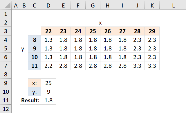
Table of Contents
- How to perform a two-dimensional lookup
- Reverse two-way lookups in a cross reference table [Excel 2016]
- Reverse two-way lookups in a cross reference table [All excel versions]
- Reverse two-way lookup in a cross reference table
- Two-dimensional lookup using two tables
- Create a hyperlink linked to the result of a two-dimensional lookup
1. How to perform a two-dimensional lookup
I have the header row (i.e. 24) value and the column (mm) value and want to return the x/y value. i.e I have 25/X and 9/Y item and want 1.8 to be returned.
(mm) 22 23 24 25 26 27 28 29
8 1.3 1.8 1.8 1.8 1.8 1.8 2.3 2.3
9 1.3 1.8 1.8 1.8 1.8 1.8 2.3 2.3
10 1.3 1.8 1.8 1.8 1.8 1.8 2.3 2.3
11 2.2 2.8 2.8 2.8 2.8 2.8 3.3 3.3thanks
You can't use VLOOKUP in this case, you need to do two different lookups to locate the value you want based on coordinates. A two-way lookup.
Formula in D11:
If the x or y value is not found the formula returns #N/A.
Explaining formula in cell D11
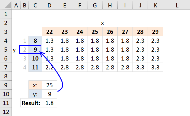
Step 1 - Find relative position of y value
MATCH(D10, C4:C7, 0)
returns 2.
Number 9 is found at the second location in this array: {8;9;10;11}.
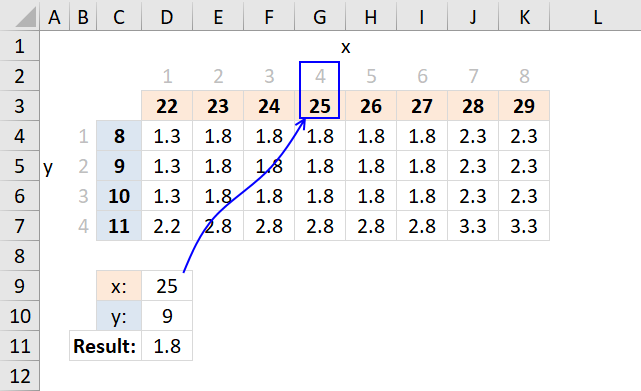
Step 2 - Find relative position of x value
MATCH(D9,D3:K3,0)
returns 4.
Number 25 is at the fourth position in the array.
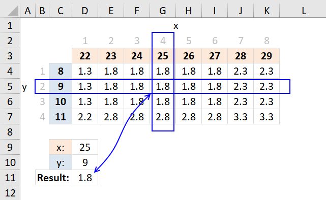
Step 3 - Get value based on coordinates
=INDEX(D4:K7,2,MATCH(D9,D3:K3,0))
becomes INDEX(D4:K7,2,4)
and returns 1.8 in cell D1.
The value is in the fourth column and the second row in cell range D4:K7. INDEX function retrieves that value based on row and column number.
2. Reverse two-way lookups in a cross-reference table [Excel 2016]
table
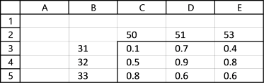
Row 2 contains variable and Column B contains another variable
The combination of 32 with 51 gives me 0.9 or cell D4
I need to report which 2 and B combinations give me values between 0.4 and 0.5. In this case, it would be 31-53 and 32-50.
I could rearrange this to be in 3 columns with the results on the last column and use something like below (The equation does not represent the example I gave.)
IFERROR(INDEX(array, SMALL(IF((min=data), ROW($B$2:$B$10)-1), ROW(A3)), COLUMN(A3)), " ")
This works but my excel table would have too many rows and the initial data set comes the other way so it would take some time to convert it. The original matrix is more compact.
I am trying to convert this equation but I am having trouble matching it to an array instead to just one column.
The following array formula returns multiple values from a cross-reference table if they meet specific criteria.
Array formula in cell H3:
If you prefer having the values in a cell each instead of concatenated values in one cell, go to this part of this article.
2.1 How to build an array formula
- Select cell H3
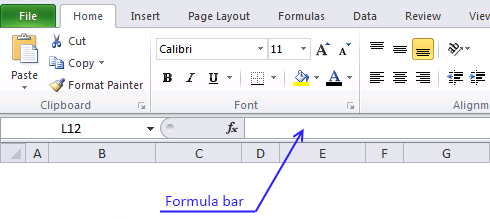
- Type the formula above in formula bar
- Press and hold CTRL + SHIFT key
- Press Enter
If you did above steps correctly excel automatically adds a beginning and ending curly bracket to the formula, like this:
![]()
Don't enter these characters yourself.
2.2 Explaining array formula in cell G3
Note, the TEXTJOIN function works only in Excel 2016. Use this formula if you have an earlier version of Excel.
Step 1 - Check which values are larger than the condition in cell H1
The less than sign and equal sign are logical operators and can be combined, the result is a boolean value True or False.
$C$3:$E$5>=$H$1
returns {FALSE, TRUE, TRUE; ... , TRUE}.
Step 2 - Check which values are smaller than the condition in cell H2
$C$3:$E$5<=$H$2
returns {TRUE,FALSE,TRUE; ... ,FALSE}.
Step 3 - Both conditions must be TRUE (AND-logic)
($C$3:$E$5>=$H$1)*($C$3:$E$5<=$H$2)
returns {0, 0, 1; 1, 0, 0; 0, 0, 0}.
Step 4 - Extract corresponding values from B3:B5 and C2:E2
The IF function returns one value if the logical test is TRUE and another value if the logical test is FALSE.
IF(logical_test, [value_if_true], [value_if_false])
IF(($C$3:$E$5>=$H$1)*($C$3:$E$5<=$H$2), $B$3:$B$5&"-"&$C$2:$E$2,"")
returns {"","","31-53";"32-50","","";"","",""},
Step 5 - Concatenate values using TEXTJOIN function
The TEXTJOIN function allows you to combine text strings from multiple cell ranges and also use delimiting characters if you want.
TEXTJOIN(delimiter, ignore_empty, text1, [text2], ...)
TEXTJOIN(",",TRUE,{"","","31-53";"32-50","","";"","",""})
returns
"31-53. 32-50" in cell H3.
Link to two-way lookups in an index table:
Looking up data in a cross reference table
2.3 Get excel *.xlsx file
Reverse two-way lookup in a cross reference table.xlsx
3. Reverse two-way lookups in a cross-reference table
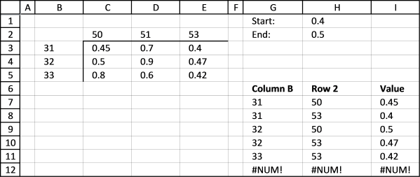
This formula is for excel versions that don't have the TEXTJOIN function or if you prefer having the values in a cell each instead of concatenated values in one cell.
Array formula in cell G7:
Array formula in cell H7:
Array formula in cell I7:
3.1 Explaining formula in cell G7
Step 1 - Check which values are larger than the condition in cell H1
The less than sign and equal sign are logical operators and can be combined, the result is a boolean value True or False.
$C$3:$E$5>=$H$1
returns {TRUE, TRUE, TRUE;... , TRUE}.
Step 2 - Check which values are smaller than the condition in cell H2
$C$3:$E$5<=$H$2
returns {TRUE, FALSE, TRUE; ... , TRUE}.
Step 3 - Both conditions must be TRUE (AND-logic)
($C$3:$E$5>=$H$1)*($C$3:$E$5<=$H$2)
returns {1, 0, 1;1, 0, 1;0, 0, 1}.
Step 4 - Create a sequence from 1 to n
The ROW function returns row numbers based on a cell reference.
ROW($B$3:$B$5)
returns {3; 4; 5}.
The MATCH function returns the relative position of an item in an array or cell reference that matches a specified value in a specific order.
MATCH(lookup_value, lookup_array, [match_type])
returns {1; 2; 3}.
Step 5 - Return corresponding row number if True
The IF function returns one value if the logical test is TRUE and another value if the logical test is FALSE.
IF(logical_test, [value_if_true], [value_if_false])
IF(($C$3:$E$5<=$H$2)*($C$3:$E$5>=$H$1)*(G7=$B$3:$B$5) ,MATCH(COLUMN($C$2:$E$2), COLUMN($C$2:$E$2)), "")
returns {1,"", 1; 2, "", 2; "", "", 3}.
Step 6 - Extract k-th smallest row number
The SMALL function returns the k-th smallest value from a group of numbers.
SMALL(array, k)
SMALL(IF(($C$3:$E$5<=$H$2)*($C$3:$E$5>=$H$1), MATCH(ROW($B$3:$B$5), ROW($B$3:$B$5)), ""), ROW(A1))
returns 1.
Step 7 - Return value based on a row number
The INDEX function returns a value from a cell range, you specify which value based on a row and column number.
INDEX(array, [row_num], [column_num])
INDEX($B$3:$B$5, SMALL(IF(($C$3:$E$5<=$H$2)*($C$3:$E$5>=$H$1), MATCH(ROW($B$3:$B$5), ROW($B$3:$B$5)), ""), ROW(A1)))
returns 31.
3.2 Get excel *.xlsx file
Reverse-two-way-lookup-in-a-cross-reference-tablev3.xlsx
4. Reverse two-way lookup in a cross-reference table
The following array formulas return a single value from a cross-reference table.
Array formula in cell E15:
Array formula in cell E16:
4.1 Explaining array formula in cell E15
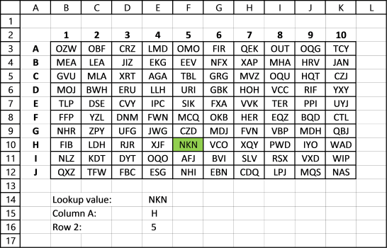
Step 1 - Check what values in cell range equals the value in E14 and return the smallest row
MIN(IF(B3:K12=E14, MATCH(ROW(B3:K12), ROW(B3:K12)), ""))
returns 5.
Step 2 - Return corresponding header value
=INDEX($A$3:$A$12, 5)
returns H.
5. Two-dimensional lookup using two tables
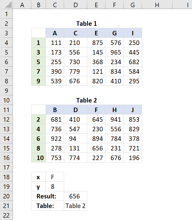
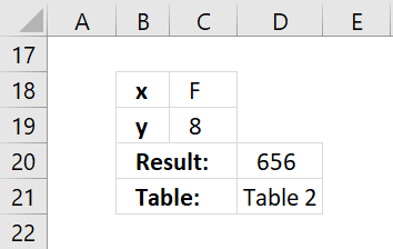
The following formula performs a two-way lookup in two different tables. The formula uses the value specified in cell C18 and performs a lookup in cell range C3:G3. It also performs a lookup in cell range B4:B8 using the value specified in cell C19. This is why it is named a two-way lookup, it performs a horizontal lookup and a vertical lookup. If matching values are found then the cell value where the intersecting row and column meet is returned to cell D20.
However, if matching values are not found then the formula automatically continues looking for values in Table2. This is what happens in the example demonstrated in the image above. "F" and 8 are found in cells E11 and B15 respectively. The result is 656.
Formula in cell D20:
If the value is not found in table 1 the formula continues to table 2. If nothing is found in table 2 as well the formula returns #N/A.
The formula does not return multiple values from different tables, in that case, check out this User defined Function:
Recommended articles
This article describes two ways to perform lookups in multiple in multiple cross reference tables simultaneously. The first one being […]
Formula in cell D21:
The formula above checks if the value is found in table 1 or table 2.
Explaining formula in cell D20
Step 1 - Find relative position of y value in table 1
The MATCH function looks for number 8 in the vertical cell range B4:B8.
MATCH(C19,B4:B8,0)
returns #N/A. The value is not found.
Step 2 - Find relative position of x value in table 1
The second MATCH function looks for "F" in the horizontal cell range C3:G3.
MATCH(C18,C3:G3,0)
returns #N/A. The value is not found.
Step 3 - Get value based on coordinates in table 1
INDEX(C4:G8,MATCH(C19,B4:B8,0),MATCH(C18,C3:G3,0))
returns #N/A. The value is not found in the first table.
Step 4 - IF error continue to table 2 and repeat
=IFERROR(INDEX(C4:G8, MATCH(C19, B4:B8, 0), MATCH(C18, C3:G3, 0)), INDEX(C12:G16, MATCH(C19, B12:B16, 0), MATCH(C18, C11:G11, 0)))
returns 656 in cell D20.
Multiple tables
It is possible to use more than two tables, simply use this template:
The formula would then be:
Get excel *.xlsx file
Two-dimensional lookup using multiple tables.xlsx
6. Create a hyperlink linked to the result of a two-dimensional lookup
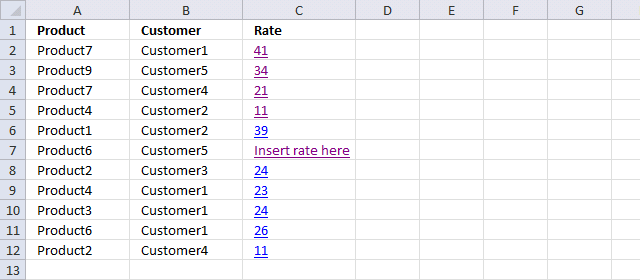
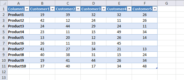
The image above shows a formula in cell C2 that searches for a value based on two conditions specified in column A and B. The image below shows an Excel Table containing values.
The formula returns a value based on a condition that matches a particular header name (horizontal lookup) and another condition that matches a value in the first column (vertical lookup), see image below.
For example, the formula in cell C2 in the image above looks for Product7 in column1 and Customer1 in Table headers and returns the intersecting value, in this case, 41 from the Excel Table. This is called a two-dimensional lookup, read this if you want to learn more: How to perform a two-dimensional lookup
The formula also creates automatically a hyperlink pointing to that particular value in the Excel Table, that is why you see values formatted as hyperlinks in column C.
This makes it really easy to find the value in the Excel Table, simply press with left mouse button on the hyperlink and you will be instantly taken to the correct value in the Excel Table.
I have a table with customers as columns & products as rows. Price may different to each customer and product. I am using the following formula to find out the rate of an item for a particular customer;
Now I want to locate/hyperlink the particular cell intersecting the customer reference and product reference.
The formula in column C searches for the product and the customer in the table below and returns the intersecting value.
Press with mouse on a value in column C and you will instantly select the returned value in the Excel Table.
Product6 / Customer5 does not have a value in the table so the formula tells you to insert a value here, see row 7 above.
Array formula in cell C2, sheet1:
You don't need to enter this formula as an array formula yf you are an Excel 365 subscriber, simply press Enter.
How to enter an array formula
- Select cell C2
- Copy (Ctrl + c) and paste (Ctrl + v) above array formula to Excel
- Press and hold CTRL + SHIFT simultaneously.
- Press Enter.
- Release all keys.
If you did it right, the formula begins and ends with curly brackets, like this:
{=array_formula}
Do not enter these characters yourself, they appear automatically.
Explaining array formula in cell C2

Excel provides a tool that can help you examine, evaluate and troubleshoot a formula, press with left mouse button on the cell that contains the formula you want to check. In this case, we are going to evaluate cell C2.
Cell C2 contains a formula that creates a hyperlink which prevents us from selecting it, if you press with left mouse button on it you will be navigated to another cell in the Excel Table. We need to use the arrow keys to select cell C2 or press with right mouse button on with the mouse to select cell C2.
Go to tab "Formulas" on the ribbon. Press with mouse on "Evaluate Formula" button to open the "Evaluate Formula" dialog box. The "Evaluate" button lets you see the calculations step by step, then press with left mouse button on "Close" button to dismiss the dialog box.
Step 1 - Find row number of the matching product value
The MATCH function returns the relative position of an item in an array or cell reference that matches a specified value in a specific order.
MATCH(lookup_value, lookup_array, [match_type])
The third argument in the function is 0 (zero), this means that it will perform an exact match. Table1[Column1] is a structured reference, in other words, a reference to a column named "Column1" in an Excel Table named Table1.
MATCH(Sheet1!A2, Table1[Column1], 0)
becomes
MATCH("Product7",{"Product1"; "Product2"; "Product3"; "Product4"; "Product5"; "Product6"; "Product7"; "Product8"; "Product9"; "Product10"}, 0)
and returns 7. "Poduct7" is the seventh value in the array counting from left to right.
Step 2 - Find column number of the matching customer value
This part of the formula calculates a number representing the column in the Excel Table that we want to extract a value from.
MATCH(Sheet1!B2, Table1[#Headers], 0)
becomes
MATCH("Customer1", {"Column1", "Customer1", "Customer2", "Customer3", "Customer4", "Customer5"}, 0)
and returns 2. "Customer1" is the second value in the array.
Step 3 - Return intersecting value
The INDEX function returns a value based on the row and column number calculated in the two previous steps.
INDEX(Table1, MATCH(Sheet1!A2, Table1[Column1], 0), MATCH(Sheet1!B2, Table1[#Headers], 0))
becomes
INDEX(Table1, 7, 2)
and returns 41. The image below shows the intersecting value based on the relative row and column number. "Relative" meaning rows and columns in the Excel Table, not in the worksheet.

Step 4 - Check if value is 0 (zero) and return intersecting value or "Insert rate"
The IF function returns text string "Insert rate here" if the formula returns a blank (nothing) and the value if it returns anything else.
IF(logical_test, [value_if_true], [value_if_false])
IF(INDEX(Table1, MATCH(Sheet1!A2, Table1[Column1], 0), MATCH(Sheet1!B2, Table1[#Headers], 0))=0, "Insert rate here", INDEX(Table1, MATCH(Sheet1!A2, Table1[Column1], 0), MATCH(Sheet1!B2, Table1[#Headers], 0)))
becomes
IF(41=0, "Insert rate here", 41)
becomes
IF(FALSE, "Insert rate here", 41)
and returns 41.
Step 5 - Calculate address to intersecting value
The ADDRESS function calculates the cell reference needed to build the hyperlink.
ADDRESS(row_num, column_num, [abs_num], [a1], [sheet_text])
"[Locate a particular cell in a table.xlsx]Sheet2!"&ADDRESS(MATCH(Sheet1!A2, Table1[[#All], [Column1]], 0), MATCH(Sheet1!B2, Table1[#Headers], 0))
becomes
"[Locate a particular cell in a table.xlsx]Sheet2!"&ADDRESS(8, 2)
becomes
"[Locate a particular cell in a table.xlsx]Sheet2!"&$B$8
and returns [Locate a particular cell in a table.xlsx]Sheet2!$B$8
Step 6 - Create hyperlink
The HYPERLINK function creates a hyperlink using the value [friendly_name] and the cell reference (link_location).
HYPERLINK(link_location, [friendly_name])
HYPERLINK("[Locate a particular cell in a table.xlsx]Sheet2!"&ADDRESS(MATCH(Sheet1!A2, Table1[[#All], [Column1]], 0), MATCH(Sheet1!B2, Table1[#Headers], 0)), IF(INDEX(Table1, MATCH(Sheet1!A2, Table1[Column1], 0), MATCH(Sheet1!B2, Table1[#Headers], 0))=0, "Insert rate here", INDEX(Table1, MATCH(Sheet1!A2, Table1[Column1], 0), MATCH(Sheet1!B2, Table1[#Headers], 0))))
becomes
HYPERLINK([Locate a particular cell in a table.xlsx]Sheet2!$B$8, 41)
and returns 41 (hyperlink) in cell C2.
Lookups category
This article demonstrates a formula that allows you to search a data set using any number of conditions, however, one […]
Two dimensional lookup category
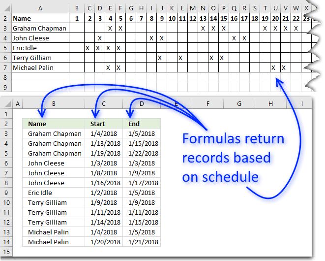
This article demonstrates ways to extract names and corresponding populated date ranges from a schedule using Excel 365 and earlier […]
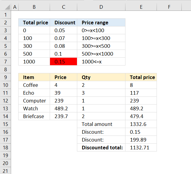
Have you ever tried to build a formula to calculate discounts based on price? The VLOOKUP function is much easier […]
Excel categories
38 Responses to “How to perform a two-dimensional lookup”
Leave a Reply
How to comment
How to add a formula to your comment
<code>Insert your formula here.</code>
Convert less than and larger than signs
Use html character entities instead of less than and larger than signs.
< becomes < and > becomes >
How to add VBA code to your comment
[vb 1="vbnet" language=","]
Put your VBA code here.
[/vb]
How to add a picture to your comment:
Upload picture to postimage.org or imgur
Paste image link to your comment.
Oscar,
Hello again, I still have trouble with this excel
(remember?
B 1 2 3 4 5 6-20
bole1 24 27 10 43 63 45
bole2 25 09 98 12 56 32
bole3 33 12 39 00 23 11
You know, in reality
I have something like this
B 1 2 3 4 5
bole1 24|| 27|| 10|| 43|| 63
bole2 25|| 09|| 98|| 12|| 56
bole3 33|| 12|| 39|| 85|| 23
D 20 30 43 50
Doll1 200|||345||231||600
Doll2 124|||232||452||320
Do you know how can I combine these 2 tables with the same INDEX?
Thanks anyway
Russel,
My answer has two index functions.
Formula in cell C14:
Get the Excel 2007 file *.xlsx
russel.xlsx
I cannot thank you enough for this.Ether way I thank you very much...
But I have office 2003 and also
when I change the value x-axis for example,it appears #NAME? error...same as if I use the formula to my example
Oscar,
I think that the function IFERROR is not supported in Office 2003
Russel,
Excel 2003 formula:
Also, if the tables are more than 2, is the same type right?
Oscar,
You are GREAT!The God of the excel...i try to convert to if(iserror)
but I forget the third Index...witch i believe make the difference!
And I think with the If(iserror is more easy for above the 3 tables right?
Russel,
thanks.
The iferror function is easier.
Oscar,
Hello again!
Is there a "logic-form" for above 3 tables?Always with the if(iserror)?
Russel,
Two index functions:
=IF(ISERROR(formula_tbl_1)), formula_tbl_2, formula_tbl_1)
Three index functions:
=IF(ISERROR(formula_tbl_1)), IF(ISERROR(formula_tbl_2)), formula_tbl_3), formula_tbl_2), formula_tbl_1)
Oscar,
I try the function,now with 4 tables!And I guess that is something like this
=IF(ISERROR(formula_tbl_1)), IF(ISERROR(formula_tbl_2)), IF(ISERROR(formula_tbl_3)), formula_tbl_4),formula_tbl_3)formula_tbl_2), formula_tbl_1)
Right?
For one more time,thank you very much!
Russel,
Yes!
I removed some brackets.
Oscar,
Great, works like a charm!
One question more,is the "formula_tbl_1" an example-shortcut of writing this
INDEX(B2:F4, MATCH(C11, A2:A4, 0), MATCH(C12, B1:F1, 0))), INDEX(B7:E8, MATCH(C11, A7:A8, 0), MATCH(C12, B6:E6)
Or there is a way, to name your formula, like named ranges?
Russel,
I simplified the formula to make it easier to read.
But you could also create named ranges for each table, I tried and it works.
i am facing a problem with two tables -
Table 1
column1 column2 column3
row1 a 1 2
row2 b 3 4
row3 c 5 6
row4 d 7 8
Table 2
column1 column2 column3
row1 a a a
row2 b b b
row3 c d
row4 d
Now i'm trying to put a formula such that from table 2, if column 1 is referred, it should then refer to table 1 and pick corresponding values from either column 1 or 2 and add the values and give results - in above case, if from table 2, column 3 is selcted, then i shoudl get the result as (1+3 = 4 or 2+4 = 6 depending on what column is required to be referred in table 1.
Hi Oscar,
You are really amazing!
Thanks a lot
Hi Oscar,
I have a cross reference table we use for shift scheduling. The x-axis is comprised of dates and the y is names. The table values indiciate whether or not the employee is scheduled to work (i.e., filled or not). Is there anyway to pull a list of names in a canned daily report based on the date and whether the cell is filled? In other words, I want to lookup the y-axis headers as opposed to the cross reference value.
Thanks,
Geoff
Geoff,
Great question!
Read this post: Shift schedule
[...] Excel, Search/Lookup, Templates on Aug.17, 2012. Email This article to a Friend Geoff asks:Hi Oscar, I have a cross reference table we use for shift scheduling. The x-axis is comprised of [...]
Says "Cannot open specified file"... Am I doing something wrong?
chrisham,
Make sure you saved the file as "Locate a particular cell in a table.xlsx".
or change the array formula to
=HYPERLINK("[yourfilename]Sheet2!"&ADDRESS(MATCH(Sheet1!A2, Table1[[#All], [Column1]], 0), MATCH(Sheet1!B2, Table1[#Headers], 0)), IF(INDEX(Table1, MATCH(Sheet1!A2, Table1[Column1], 0), MATCH(Sheet1!B2, Table1[#Headers], 0))=0, "Insert rate here", INDEX(Table1, MATCH(Sheet1!A2, Table1[Column1], 0), MATCH(Sheet1!B2, Table1[#Headers], 0))))
Oscar -
Can you change the formula so that the hyperlink address will return the correct value if the source table does not start at A1? For example, my lookup range starts at $L$20 and the value may be at $N$22 but the ADDRESS function for the hyperlink returns $C$3 since it's the 3rd row and 3rd column in the lookup range.
Got it (at least one way)...
Match criteria are on worksheet Formulas!D99 and !E99
Lookup range is on worksheet Sources!L11:N62 not including column headers in row 10.
=HYPERLINK(CELL("address", OFFSET(Sources!$L$11,MATCH(Formulas!$D99,Sources!$L$11:$L$62,0)-1, MATCH(Formulas!$E99, Sources!$L$10:$N$10, 0)-1)), IF(OFFSET(Sources!$L$11, MATCH(Formulas!$D99, Sources!$L$11:$L$62, 0)-1, MATCH(Formulas!$E99, Sources!$L$10:$N$10, 0)-1)=0, "No value found", OFFSET(Sources!$L$11, MATCH(Formulas!$D99, Sources!$L$11:$L$62, 0)-1, MATCH(Formulas!$E99, Sources!$L$10:$N$10, 0)-1)))
Excel forces the use of the CELL-OFFSET combination to return the actual address of the cell rather than its relative row and column position in the range. But it has the advantage that the CELL function returns the full path of the file and worksheet so you don't have to put them in square brackets for the HYPERLINK argument if you're in the same spreadsheet.
Now if only Excel would come up with an IFZERO function similar to IFERROR so that you don't have to duplicate your formula in the logical test and the outcome! Even better a generic
IFVALUE(test_condition,if_true,if_false)
So testing the above code for a zero value would give IFVALUE(0,,"Insert rate here"). I tried a UDF but it wouldn't refresh as nicely as a native Excel function.
GMF,
Can you change the formula so that the hyperlink address will return the correct value if the source table does not start at A1?
Great question!
I created this formula:
=HYPERLINK("[Locate-a-particular-cell-in-a-table.xlsx]Sheet2!"&ADDRESS(MATCH(Sheet1!A2, Table1[[#All], [Column1]], 0)+CELL("row", Table1)-2, MATCH(Sheet1!B2, Table1[#Headers], 0)+CELL("col", Table1)-1), IF(INDEX(Table1, MATCH(Sheet1!A2, Table1[Column1], 0), MATCH(Sheet1!B2, Table1[#Headers], 0))=0, "Insert rate here", INDEX(Table1, MATCH(Sheet1!A2, Table1[Column1], 0), MATCH(Sheet1!B2, Table1[#Headers], 0))))
Get the Excel *.xlsx file
Locate-a-particular-cell-in-a-tablev2.xlsx
Thanks for sharing!
GMF,
Now if only Excel would come up with an IFZERO function similar to IFERROR so that you don't have to duplicate your formula in the logical test and the outcome! Even better a generic
IFVALUE(test_condition,if_true,if_false)
Another great question!
Formula:
=HYPERLINK("[Locate-a-particular-cell-in-a-table.xlsx]Sheet2!"&ADDRESS(MATCH(Sheet1!A2, Table1[[#All], [Column1]], 0)+CELL("row", Table1)-2, MATCH(Sheet1!B2, Table1[#Headers], 0)+CELL("col", Table1)-1), IFERROR(1/(1/(INDEX(Table1, MATCH(Sheet1!A2, Table1[Column1], 0), MATCH(Sheet1!B2, Table1[#Headers], 0)))), "Insert rate here"))
Get the Excel *.xlsx file
Locate-a-particular-cell-in-a-tablev3.xlsx
The IFERROR(1/0) test is good for numeric values but generates the error option if you're returning text (for example, a lookup of tax rates could provide a text range ["1.6% - 7.4%"] for 2013 Idaho state taxes whereas Illinois has a flat 5% formatted as a number). I guess you'd have to tailor the error handling to the type of data you expect to return.
Mere quibbles considering the usefulness of the overall post!
[…] https://www.get-digital-help.com/reverse-two-way-lookup-in-a-cross-reference-table/ […]
Hi Oscar,
Thank you very much.
Is there a way to report each combination with its corresponding results so in the example provided you would see
Column J Column K Column L
31 53 0.4
32 50 0.5
or
Column J Column K
31-53 0.4
32-50 0.5
Thanks Again.
Polar
(P.S Sorry this is a repost from the old thread. Just making sure I am not confusing things).
Polar,
Yes, it is possible. Read this.
Thank you!
This is exactly what I have been looking for except for I need to have in the horizontal (x)cell say 2000 next to it 3000 and 4000 so on. And the same on the vertical (y) and cross reference it. but if I put in 2859 x value and 2679 in the y value. How do I do it so it goes up to the next highest value (3000) between the 2000 and 3000. I have 2003 excel. I have a paper chart and wanting to put it into a spreadsheet. Thanks Allan.
Alan White,
Try this:
Formula in cell C10:
=INDEX(C3:E5, MATCH(C9, B3:B5)+1, MATCH(C8, C2:E2)+1)
How would I go about looking up data in a cross-reference table.
I have the header row (i.e. 25) value and the column (mm) value and want to return the x/y value. i.e I have 0.25/X and 0.48/Y item and want 1.6 to be returned.
(mm) width 10~20 20.1~30 30.1~40 40.1~50
0.2~0.45 1.3 1.8 2.1 3.5
0.46~0.60 1.4 1.6 1.8 2.3
0.61~0.70 1.5 1.7 1.6 2.1
0.71~0.80 0.7 1.1 2.2 3.1
Sergio,
Formula in cell C10:
=INDEX(C3:F6,MATCH(C9,B3:B6)+1,MATCH(C8,C2:F2)+1)
Hi Oscar,
Not sure if you can help here:
How do I look up (search for) a value (text) in a table and return the cell reference. Example: search for the name "John" in B1:F24, and if found, return cell address, say D6. Preferably, I'd like to find "John" and return the only the ROW number, in my example 6. I could then use this ROW value in INDEX function.
Apologies, if this is simple, but i've almost lost it trying to figure it out for the past few days. Thanks.
Gerry,
No need to apologize, I am happy to help you out.
Try this array formula to get the row number:
=MIN(IF(B1:F24="John",ROW(B1:F24,""))
Press CTRL + SHIFT + ENTER to create an array formula.
Hello, First of All Thank you so much for sharing your Knowledge, makes a happier world. Second I want to do the opposite of this topic. And I do not have a clue if it is possible. I want to have a list of "things" with to values "X" and "Y" that will help as a coordinates. Then in a second sheet I want to have the first row labeled from "0" to "n" and the first column labeled from "0" to "n". In this second sheet I want to appear in the cell the name of the "Thing" in the square were is crossing the value of the column "x" and "y". The list will change all the time and will be given different values. And in an advance feature will be to calculate how far is the "thing 1" from "thing 2" on a straight line trajectory.
_______________
Thing | x | y |
---------------
house | 5 | 5 |
park | 1 | 1 |
---------------
Second sheet:
______________________
|park| | | | |
----------------------
| | | | | |
----------------------
| | | | | |
----------------------
| | | | | |
----------------------
| | | | |house|
----------------------
Thank you so much for your time and help.
Regards,
Art
If there are be the same data in y_header (i.e several 9) how i can extract a list of data?