How to use the MAP function

What is the MAP function?
The MAP function is a new Excel 365 function that requires the LAMBDA function to work. It passes all values in an array to a LAMBDA function, which then calculates new values based on a formula you specify. It finally returns an array with the same size as the original array.
In other words, the process involves applying a specified formula to every element in an array or range. When multiple arrays are used, values are paired up based on their positions across the arrays. This pairing allows the formula to be applied to corresponding elements from each array. The following examples will illustrate this concept thoroughly.
Table of Contents
1. Introduction
What is an array in Excel?
An array in Excel is a collection of values arranged in rows and columns. It can be thought of as a table or a grid of data.
There are two types of arrays. One-dimensional arrays: A single row or column of data. Two-dimensional arrays: Data organized in both rows and columns.
There are two types of array formulas: The first type returns a single value and the second type returns multiple values. An array formula is a formula that can perform multiple calculations on one or more sets of values.
Excel 365 subscribers have access to dynamic array formulas, a powerful feature that automatically adjusts its output range. These formulas populate the initial target cell and expand into neighboring cells as needed, adapting their size based on the formula's result. This automatic expansion and contraction of the output range is the key characteristic that gives them the name "dynamic" array formulas. The process of extending results into adjacent cells is known as "spilling.
Excel processes arrays in RAM allowing for rapid computations. However, when array sizes exceed available memory, Windows may resort to using virtual memory on the hard drive or SSD. This fallback to disk storage significantly slows down calculations, as accessing data from these devices is much slower than from RAM.
What is the LAMBDA function?
The MAP function uses the LAMBDA function as its second argument to define how each cell in the array should be calculated. This combination allows you to perform cumulative calculations across a range of values.
The LAMBDA function is required in the MAP function, you can't leave it out. Read more: LAMBDA function
2. Syntax
MAP(array_1, lambda_or_array<#>)
| array_1 | Required. A cell reference to a cell range or an array. |
| array_n | Optional. A cell reference to a cell range or an array. |
| lambda_or_array | Required. A LAMBDA function, it must be the last argument in the MAP function. Each array uses a different parameter in the LAMBDA function. |
3. Example 1
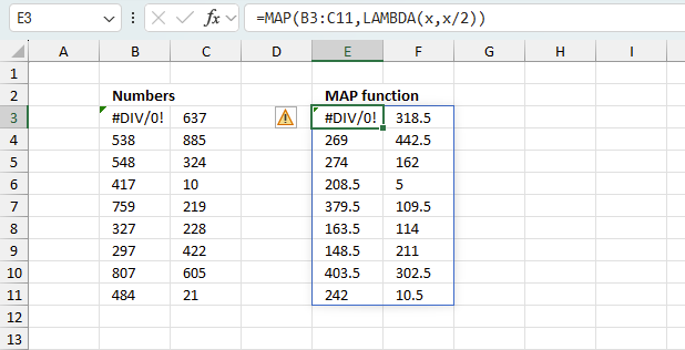
This example shows how to divide each number in the array B3:C11 by 2. The source data is in cell range B3:C11 and the result is displayed in cell range E3:F11.
Formula in cell E3:
This formula is an Excel 365 dynamic array formula meaning it spills values to adjacent cells as far as needed. This is a simple demonstration of the MAP function, I know that the formula can be made a lot smaller using only the division operator.
Explaining the formula
Step 1 - Build LAMBDA function
The LAMBDA function build custom functions without VBA, macros or javascript.
Function syntax: LAMBDA([parameter1, parameter2, …,] calculation)
The LAMBDA function is iterated as many times as there are values in cell range B3:C11.
LAMBDA(x,x/2)
The first argument specifies the parameter, the second argument lets you build a formula.
Step 2 - Pass values to the LAMBDA function
The MAP function lets you pass arrays to the LAMBDA function.
MAP(B3:C11, LAMBDA(x,x/2))
The first number is 771 in cell range B3:C11. 771/2 equals 385.5
It then continues with the remaining values returning an array with a size that matches the original array (B3:C11).
4. MAP Function Example 2

This example demonstrates how to pass two arrays to the LAMBDA function. The LAMBDA function adds the first value in the first array B3:B11 to the first value in the second array. In other words, the calculations are based on the value's position in the array.
Formula in cell E3:
The first value in the first array named x (B3) is 771, the first value in the second array y (C3) is 637. The LAMBDA function performs addition based on these values: 771 + 637 equals 1408.
The formula then continues to the next value pairs and continues to add the numbers. For example, the second value is 538 in the first array (B3:B11) and the second value in the second array (C3:C11) is 885. The formula returns 1423 in cell E4 based on 538 + 885 = 1423
Explaining the formula
Step 1 - Build the LAMBDA function
The LAMBDA function build custom functions without VBA, macros or javascript.
Function syntax: LAMBDA([parameter1, parameter2, …,] calculation)
LAMBDA(x,y,x+y)
The two first parameters specifies which parameters to use, they correspond to the arrays in the MAP function.
x+y is the formula in the LAMBDA function.
Step 2 - Pass values to the LAMBDA function
MAP(B3:B11,C3:C11,LAMBDA(x,y,x+y))
x - B3:B11
y - C3:C11
x + y = B3:B11 + C3:C11
5. MAP Function Example 3

A data table containing three columns and 9 rows contains information about a survey. How many numbers in each row exceed 500?
The source data is located in cell range B3:D11, it contains random integers between 1 and 1000. The formula in cell F3 counts the number of integers that meet the condition.
Formula in cell F3:
This formula is an Excel 365 dynamic array formula meaning it spills values to adjacent cells as far as needed. The first values in each cell range B3:B11, C3:C11, and D3:D11 are 771, 637, and 948. They all meet the given condition. This results in 3 in cell F3 meaning there are three numbers larger than 500 in cells B3, C3, and D3.
This is not the case in cells B4, C4, and D4. Only two are larger than 500. They are 538 and 885. 445 is smaller than 500. The formula continues to process each pairs until all values are evaluated.
Explaining formula
Step 1 - Specify arguments in the MAP function
MAP(B3:B11,C3:C11,D3:D11,LAMBDA(...)))
Step 2 - Specify arguments in the LAMBDA function
There are three cell references in the MAP function which must correspond to 3 variables in the LAMBDA function. I named them x, y, and z.
LAMBDA(x,y,z,...)
Step 3 - Define the condition
The larger than character > allows you to create a condition that evaluates to TRUE if numbers are larger than 500. We need to specify all three variables.
x>500,y>500,z>500
Step 4 - Count numbers larger than 500
The SUM function allows you to add numerical values, the function returns the sum in the cell it is entered in. The SUM function is cleverly designed to ignore text and boolean values, adding only numbers.
Function syntax: SUM(number1, [number2], ...)
SUM(x>500,y>500,z>500)
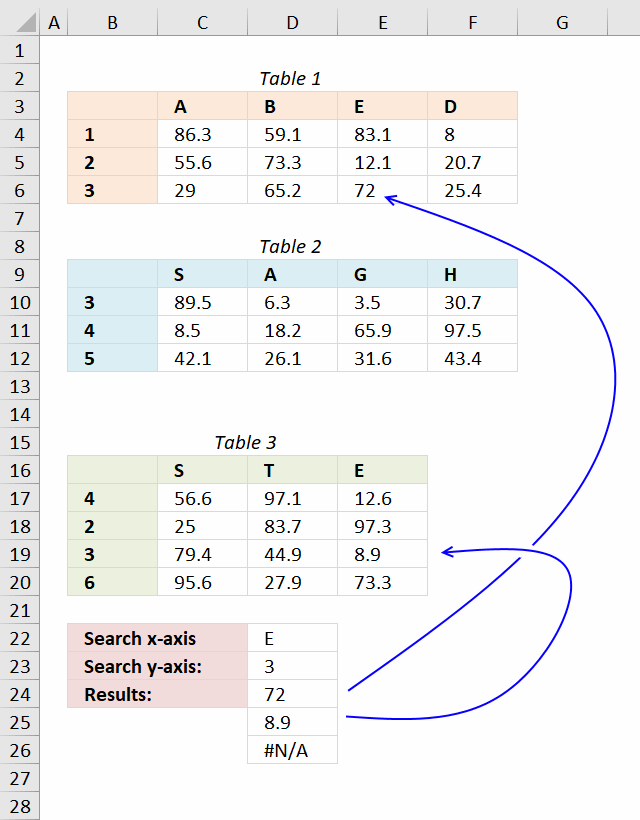
7. Two-way lookup using multiple tables

This example demonstrates how to perform lookups in multiple in multiple cross reference tables simultaneously using an Excel 365 LAMBDA function.
The first and second conditions are in cells D23 and D24 respectively. The cell references populates cells D19 to D21. The result is shown in cell D26, it spills values to cells below as far as needed.
Excel 365 formula in cell D26:
The formula returns a value for each cell reference, an #N/A error is displayed if at least one condition is not found.
Explaining formula
Step 1 - Convert string to cell reference
The INDIRECT function returns the cell reference based on a text string and shows the content of that cell reference.
Function syntax: INDIRECT(ref_text, [a1])
INDIRECT(a)
Step 2 - Get the first row
The INDEX function returns a value or reference from a cell range or array, you specify which value based on a row and column number.
Function syntax: INDEX(array, [row_num], [column_num])
INDEX(INDIRECT(a),1,0)
A 0 (zero) in the column argument lets you get all values in row 1. This is also true if you use a 0 (zero) in the row argument, however, this returns all values in a column in the specified cell range.
Step 3 - Match first condition
The MATCH function returns the relative position of an item in an array that matches a specified value in a specific order.
Function syntax: MATCH(lookup_value, lookup_array, [match_type])
MATCH(D23,INDEX(INDIRECT(a),1,0),0)
Step 4 - Get value in cross reference table based on first and second condition
The INDEX function returns a value or reference from a cell range or array, you specify which value based on a row and column number.
Function syntax: INDEX(array, [row_num], [column_num])
INDEX(INDIRECT(a),MATCH(D23,INDEX(INDIRECT(a),1,0),0),MATCH(D24,INDEX(INDIRECT(a),0,1),0))

The first condition is used in the horizontal lookup, the second condition is used in the vertical lookup.
Step 5 - Build LAMBDA function
The LAMBDA function build custom functions without VBA, macros or javascript.
Function syntax: LAMBDA([parameter1, parameter2, …,] calculation)
LAMBDA(a,INDEX(INDIRECT(a),MATCH(D23,INDEX(INDIRECT(a),1,0),0),MATCH(D24,INDEX(INDIRECT(a),0,1),0)))
The LAMBDA function is a requirement in order to use the MAP function in step 6.
Step 6 - Pass cell refs to LAMBDA function
The MAP function passes all values in an array to a LAMBDA function, the LAMBDA function calculates new values based on a formula you specify. It then returns an array with the same size as the original array.
Function syntax: MAP(array1, lambda_or_array<#>)
MAP(D19:D21,LAMBDA(a,INDEX(INDIRECT(a),MATCH(D23,INDEX(INDIRECT(a),1,0),0),MATCH(D24,INDEX(INDIRECT(a),0,1),0))))
The MAP function allows you to iterate or loop through each cell reference and return a corresponding value.
8. Two-way lookup using multiple tables - User Defined Function
A User defined function is a custom function anyone can use, simply copy the VBA code and paste to your workbooks code module and you are good to go.
The custom function demonstrated in this article accepts an arbitrary number of range arguments (table ranges). The custom function returns the first match in each table if there is a match.
Array formula in cell C24:C26:
How to enter an array formula
- Select cell range C24:C26
- Copy above formula
- Paste formula
- Press and hold Ctrl + Shift
- Press Enter once
- Release all keys
User Defined Function Syntax
SEARCHMULTIPLETBL(xaxis, yaxis, cellrange1, [cellrange2])
Arguments
| Parameter | Text |
| xaxis | Required. The x-axis condition you want to search for. |
| yaxis | Required. The y-axis condition you want to search for. |
| cellrange1 | Required. The range you want to add. |
| [cellrange2] | Optional. You may have up to 255 additional argument cell ranges. |
VBA Code:
'Name function and arguments
Function SEARCHMULTIPLETBL(xaxis As Variant, yaxis As Variant, ParamArray cellranges() As Variant)
'Declare variables and data types
Dim i As Integer, x As Variant, y As Variant
Dim temp() As Variant, xrange As Range, yrange As Range
'Redimension array variable temp so it may grow
ReDim temp(0)

'Iterate through all cell ranges
For i = LBound(cellranges) To UBound(cellranges)
    'Enable error handling
    On Error Resume Next
    'Save first row to xrange object
    Set xrange = cellranges(i).Rows(1)
    'Save first column to yrange object
    Set yrange = cellranges(i).Columns(1)
        'Find position of matching value in row and column
        x = Application.WorksheetFunction.Match(xaxis, xrange, 0)
        y = Application.WorksheetFunction.Match(yaxis, yrange, 0)
        'If found an error is not returned and Err.Number becomes 0 (zero)
        If Err.Number = 0 Then
            temp(UBound(temp)) = cellranges(i).Rows(y).Columns(x).Value
            ReDim Preserve temp(UBound(temp) + 1)
        Else
            'Disable error handling
            On Error GoTo 0
        End If
'Continue with next cell range
Next i
'Remove last container in array
ReDim Preserve temp(UBound(temp) - 1)
'Return values in temp array rearranged (transposed)
SEARCHMULTIPLETBL= Application.Transpose(temp)

End Function
Where to copy vba code?
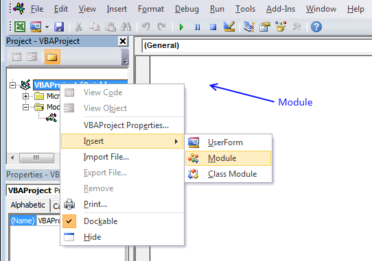
- Press Alt-F11 to open the Visual Basic Editor
- Press with left mouse button on Module on the Insert menu
- Copy and paste vba code.
- Exit visual basic editor

9. Function not working
The MAP function returns
- #NAME? error if you misspell the function name or use undefined variables.
- propagates errors, meaning that if the input contains an error (e.g., #VALUE!, #REF!, #DIV/0!), the function will return the same error.
9.1 Troubleshooting the error value
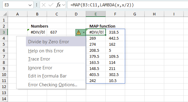
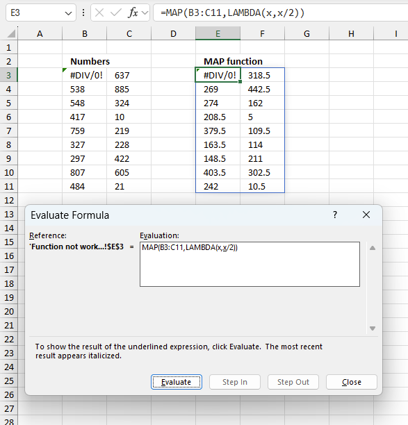
When you encounter an error value in a cell a warning symbol appears, displayed in the image above. Press with mouse on it to see a pop-up menu that lets you get more information about the error.
- The first line describes the error if you press with left mouse button on it.
- The second line opens a pane that explains the error in greater detail.
- The third line takes you to the "Evaluate Formula" tool, a dialog box appears allowing you to examine the formula in greater detail.
- This line lets you ignore the error value meaning the warning icon disappears, however, the error is still in the cell.
- The fifth line lets you edit the formula in the Formula bar.
- The sixth line opens the Excel settings so you can adjust the Error Checking Options.
Here are a few of the most common Excel errors you may encounter.
#NULL error - This error occurs most often if you by mistake use a space character in a formula where it shouldn't be. Excel interprets a space character as an intersection operator. If the ranges don't intersect an #NULL error is returned. The #NULL! error occurs when a formula attempts to calculate the intersection of two ranges that do not actually intersect. This can happen when the wrong range operator is used in the formula, or when the intersection operator (represented by a space character) is used between two ranges that do not overlap. To fix this error double check that the ranges referenced in the formula that use the intersection operator actually have cells in common.
#SPILL error - The #SPILL! error occurs only in version Excel 365 and is caused by a dynamic array being to large, meaning there are cells below and/or to the right that are not empty. This prevents the dynamic array formula expanding into new empty cells.
#DIV/0 error - This error happens if you try to divide a number by 0 (zero) or a value that equates to zero which is not possible mathematically.
#VALUE error - The #VALUE error occurs when a formula has a value that is of the wrong data type. Such as text where a number is expected or when dates are evaluated as text.
#REF error - The #REF error happens when a cell reference is invalid. This can happen if a cell is deleted that is referenced by a formula.
#NAME error - The #NAME error happens if you misspelled a function or a named range.
#NUM error - The #NUM error shows up when you try to use invalid numeric values in formulas, like square root of a negative number.
#N/A error - The #N/A error happens when a value is not available for a formula or found in a given cell range, for example in the VLOOKUP or MATCH functions.
#GETTING_DATA error - The #GETTING_DATA error shows while external sources are loading, this can indicate a delay in fetching the data or that the external source is unavailable right now.
9.2 The formula returns an unexpected value
To understand why a formula returns an unexpected value we need to examine the calculations steps in detail. Luckily, Excel has a tool that is really handy in these situations. Here is how to troubleshoot a formula:
- Select the cell containing the formula you want to examine in detail.
- Go to tab “Formulas” on the ribbon.
- Press with left mouse button on "Evaluate Formula" button. A dialog box appears.
The formula appears in a white field inside the dialog box. Underlined expressions are calculations being processed in the next step. The italicized expression is the most recent result. The buttons at the bottom of the dialog box allows you to evaluate the formula in smaller calculations which you control. - Press with left mouse button on the "Evaluate" button located at the bottom of the dialog box to process the underlined expression.
- Repeat pressing the "Evaluate" button until you have seen all calculations step by step. This allows you to examine the formula in greater detail and hopefully find the culprit.
- Press "Close" button to dismiss the dialog box.
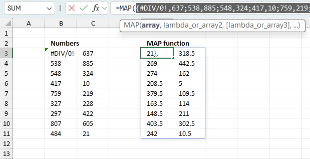
There is also another way to debug formulas using the function key F9. F9 is especially useful if you have a feeling that a specific part of the formula is the issue, this makes it faster than the "Evaluate Formula" tool since you don't need to go through all calculations to find the issue.
- Enter Edit mode: Double-press with left mouse button on the cell or press F2 to enter Edit mode for the formula.
- Select part of the formula: Highlight the specific part of the formula you want to evaluate. You can select and evaluate any part of the formula that could work as a standalone formula.
- Press F9: This will calculate and display the result of just that selected portion.
- Evaluate step-by-step: You can select and evaluate different parts of the formula to see intermediate results.
- Check for errors: This allows you to pinpoint which part of a complex formula may be causing an error.
The image above shows cell reference B3:C11 converted to hard-coded value using the F9 key. The MAP function requires non-error values which is not the case in this example. We have found what is wrong with the formula.
Tips!
- View actual values: Selecting a cell reference and pressing F9 will show the actual values in those cells.
- Exit safely: Press Esc to exit Edit mode without changing the formula. Don't press Enter, as that would replace the formula part with the calculated value.
- Full recalculation: Pressing F9 outside of Edit mode will recalculate all formulas in the workbook.
Remember to be careful not to accidentally overwrite parts of your formula when using F9. Always exit with Esc rather than Enter to preserve the original formula. However, if you make a mistake overwriting the formula it is not the end of the world. You can “undo” the action by pressing keyboard shortcut keys CTRL + z or pressing the “Undo” button
9.3 Other errors
Floating-point arithmetic may give inaccurate results in Excel - Article
Floating-point errors are usually very small, often beyond the 15th decimal place, and in most cases don't affect calculations significantly.
'MAP' function examples
The following article has a formula that contains the MAP function.
Functions in 'Logical' category
The MAP function function is one of 16 functions in the 'Logical' category.
Excel function categories
Excel categories
5 Responses to “How to use the MAP function”
Leave a Reply
How to comment
How to add a formula to your comment
<code>Insert your formula here.</code>
Convert less than and larger than signs
Use html character entities instead of less than and larger than signs.
< becomes < and > becomes >
How to add VBA code to your comment
[vb 1="vbnet" language=","]
Put your VBA code here.
[/vb]
How to add a picture to your comment:
Upload picture to postimage.org or imgur
Paste image link to your comment.
I get errors when I change C17 and 18. And when I change D6 to "E" the results are 72,42.1 and 8.9. it appears they should be 72, 31.6, and 8.9. Why is the second number returned under results "42.1"? please help me understand.
Steve,
You are right, there was something wrong with the code.
I have changed the vba code and uploaded a new file.
Many thanks for commenting!
Wow!!! Awesome,
Thanks for sharing this extremely useful logic.
I set up the data table above and have tested the Function. If the x & y value are in the first table (Table 1), everything works fine. If the data is not in the first table, but the second or third table, then it returns "#VALUE!" Is there something I am doing wrong or is this a possible bug in the function?
Bogey,
you are right, it is a bug.
I have updated this article and the attached file.
Thank you for telling me.
/Oscar