Lookup multiple values across columns and return a single value
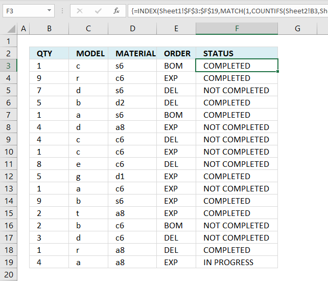
Table of Contents
1. Lookup multiple values across columns and return a single value
This article demonstrates how to get a value from a dataset based on multiple conditions across multiple columns.
ORDER MODEL MATERIAL QTY STATUS
BOM a s6 1 COMPLETED
BOM b c6 2 NOT COMPLETED
BOM c s6 1 COMPLETED
DEL d c6 3 NOT COMPLETED
EXP a a8 4 IN PROGRESS
DEL b d2 5 COMPLETED
DEL c c6 4 NOT COMPLETED
DEL d s6 7 NOT COMPLETED
DEL e c6 8 NOT COMPLETED
DEL r a8 1 COMPLETED
EXP g d1 5 COMPLETED
EXP r c6 9 COMPLETED
EXP t a8 2 COMPLETED
EXP a c6 1 NOT COMPLETED
EXP b s6 9 COMPLETED
EXP c c6 1 NOT COMPLETED
EXP d a8 4 NOT COMPLETED
S.Babu
Sheet1 - Data

Sheet2 - Criteria and result

The following array formula uses the corresponding values in column A, B, C and D to do a lookup in Sheet1 and return a value in column E.
Array formula in cell E2, sheet2:
Watch a video explaining formula above
Recommended article:
Recommended articles
This article demonstrates a formula that extracts values from a column based on a date range criteria and another condition. […]
The following article demonstrates how to do a lookup and return a sorted list:
Recommended articles
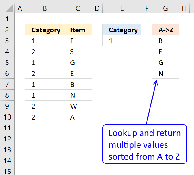
This article demonstrates how to extract multiple values based on a search value and display them sorted from A to […]
How to create an array formula
- Copy above array formula
- Double press with left mouse button on cell E2
- Paste array formula
- Press and hold Ctrl + Shift simultaneously
- Press Enter once
- Release all keys
Recommended articles

Array formulas allows you to do advanced calculations not possible with regular formulas.
How to copy array formula
- Select cell E2
- Copy cell (Ctrl + c)
- Select cell E3:E20
- Paste (Ctrl + v)
Explaining array formula in cell E2
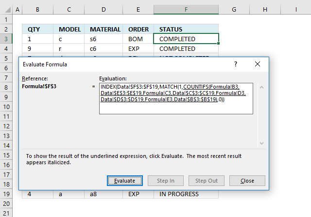
I recommend that you use the "Evaluate Formula" feature in Excel to troubleshoot or to simply understand how a formula works.
Select the cell containing the formula you want to evaluate, go to tab "Formulas" on the ribbon. Press with mouse on "Evaluate Formula" button to start evaluating.
A dialog box appears, press with left mouse button on the "Evaluate" button to go through the formula calculations step by step.
Step 1 - Count the number of cells by a given set of criteria
The COUNTIFS function can work with up to 127 argument pairs:
COUNTIFS(criteria_range1, criteria1, [criteria_range2, criteria2]…)
There are four criteria and the COUNTIFS function requires eight arguments, in order to get an array of values that we can use the second argument in each pair is a cell range.
You are probably not used to this setup but it works fine, the array allows you to identify where the match is or in other words where all criteria match.
COUNTIFS(Sheet2!A2, Sheet1!$D$2:$D$18, Sheet2!B2, Sheet1!$B$2:$B$18, Sheet2!C2, Sheet1!$C$2:$C$18, Sheet2!D2, Sheet1!$A$2:$A$18)
returns the following array {0, 0, 1, ... , 0}.
This array tells us that the match is in row 3 because 1 is in the third position in the array. Note that all criteria must match in order to return 1.
Step 2 - Return the relative position of an item in an array that matches a specified value
The MATCH function returns the relative position of a value in a cell range or array.
MATCH(1, COUNTIFS(Sheet2!A2, Sheet1!$D$2:$D$18, Sheet2!B2, Sheet1!$B$2:$B$18, Sheet2!C2, Sheet1!$C$2:$C$18, Sheet2!D2, Sheet1!$A$2:$A$18), 0)
becomes
MATCH(1, {0, 0, 1, ..., 0}, 0)
and returns 3. Value 1 is found in the third position in the array.
Step 3 - Return the value of a cell at the intersection of a particular row and column
The INDEX function returns a value based on a row and column number, there is only a row number in this case so you can omit the column argument.
INDEX(cell_reference, [row_num], [column_num])
The first argument is the cell reference from which you want to get a specific value from.
INDEX(Sheet1!$E$2:$E$18, MATCH(1, COUNTIFS(Sheet2!A2, Sheet1!$D$2:$D$18, Sheet2!B2, Sheet1!$B$2:$B$18, Sheet2!C2, Sheet1!$C$2:$C$18, Sheet2!D2, Sheet1!$A$2:$A$18), 0))
becomes
INDEX(Sheet1!$E$2:$E$18, 3)
and returns "COMPLETED" in cell E2.
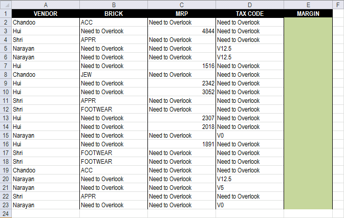
2. Lookup using multiple conditions
Debraj Roy asks:Hi Oscar,
I failed to search for "Ask" Section.. so submitting my query here.. Apologize for hijacking someones post,, and also for cross-post..
https://chandoo.org/forums/topic/lookup-using-multiple-condition
Can You please help me to create a drag-able FORMULA to get Margin.. via multiple Condition..
* Each Vendor has only one type of MARGIN decider (MRP or BRICK or TAX Code)
* According to Margin decider, I need to get MARGIN for the VENDOR..
i.e Vendor 1 (Chandoo) 's Margin Decider is BRICK..
If brick is ACC then Margin is 548, if Brick is JEW then Margin is 786.. (Check Table2 for lookupArea and Margin Decider..
LookUpArea..
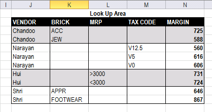
* suggestion for changing Design of LookUpArea's is appreciable.
* use of HELPER column is also acceptable..
https://dl.dropbox.com/u/78831150/Excel/MultipleLookup.xlsx
You can get the VBA version for your reference..
https://dl.dropbox.com/u/78831150/Excel/MultipleLookup.xlsm
Regards,
Deb
Answer:
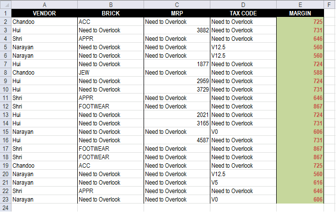
Array formula in cell E2:
How to enter an array formula
- Select cell E2
- Paste array formula to formula bar
- Press and hold CTRL + SHIFT
- Press Enter
How to copy array formula
- Select cell E2
- Copy cell E2 (Ctrl + c)
- Select cell range E3:E23
- Paste (Ctrl + v)
Explaining array formula in cell E2
Step 1 - Determine which cell range to use
The less than an larger than signs combined checks if a value is not equal to another value, the result si a boolean value TRUE or FALSE.
B2:D2<>"Need to Overlook"
returns {TRUE, FALSE, FALSE}
Step 2 - Determine which cell range to use
The MATCH function returns the relative position of an item in an array that matches a specified value in a specific order.
Function syntax: MATCH(lookup_value, lookup_array, [match_type])
MATCH(TRUE, B2:D2<>"Need to Overlook", 0)
returns 1.
Step 3 - Return cell reference
The INDEX function returns a value or reference from a cell range or array, you specify which value based on a row and column number.
Function syntax: INDEX(array, [row_num], [column_num])
INDEX((B2, C2, D2), , , MATCH(TRUE, B2:D2<>"Need to Overlook", 0))
returns cell reference B2
Step 4 - Find a matching row
The COUNTIFS function calculates the number of cells across multiple ranges that equals all given conditions.
Function syntax: COUNTIFS(criteria_range1, criteria1, [criteria_range2, criteria2]…)
COUNTIFS(INDEX((B2, C2, D2), , , MATCH(TRUE, B2:D2<>"Need to Overlook", 0)), INDEX(($K$3:$K$11, $L$3:$L$11, $M$3:$M$11), , , MATCH(TRUE, B2:D2<>"Need to Overlook", 0)), A2, $J$3:$J$11)
returns {1;0;0;0;0;0;0;0;0}.
Step 5 - Calculate the relative position of row
The MATCH function returns the relative position of an item in an array that matches a specified value in a specific order.
Function syntax: MATCH(lookup_value, lookup_array, [match_type])
MATCH(1, COUNTIFS(INDEX((B2, C2, D2), , , MATCH(TRUE, B2:D2<>"Need to Overlook", 0)), INDEX(($K$3:$K$11, $L$3:$L$11, $M$3:$M$11), , , MATCH(TRUE, B2:D2<>"Need to Overlook", 0)), A2, $J$3:$J$11), 0)
becomes
MATCH(1, {1;0;0;0;0;0;0;0;0}, 0)
and returns 1.
Step 6 - Return margin value
The INDEX function returns a value or reference from a cell range or array, you specify which value based on a row and column number.
Function syntax: INDEX(array, [row_num], [column_num])
INDEX($N$3:$N$11, MATCH(1, COUNTIFS(INDEX((B2, C2, D2), , , MATCH(TRUE, B2:D2<>"Need to Overlook", 0)), INDEX(($K$3:$K$11, $L$3:$L$11, $M$3:$M$11), , , MATCH(TRUE, B2:D2<>"Need to Overlook", 0)), A2, $J$3:$J$11), 0))
returns 725 in cell E2.
3. Lookup a date range and a condition - return multiple values
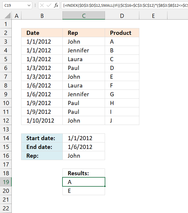
Jason C asks:I have a set of data, like the one you used in the original example that also has a column for the date of the transaction. I would like my Index-type formula to search for both the main item (the rep's name) and also if the date of the transaction falls in the date range).
Start Date: 11/26/2012
End Date: 11/30/2012 (both entered by the user)
Rep: John
Then the results, in each row/column of the 'result' section (INDEX formula results) would show results for John that occurred from 11/26 to 11/30 (including both dates).
Thanks for any help with the formula for that.
Jason
The image above demonstrates a formula in cell range B18:B19 that extracts values from column C if the corresponding value in column B is between two given dates and the corresponding value in column A matches a specified value.
The following formula is for earlier Excel versions, array formula in cell B18:
3.1 How to create an array formula
- Copy above array formula.
- Double press with left mouse button on cell E2, the prompt appears.
- Paste array formula.
- Press and hold Ctrl + Shift simultaneously.
- Press Enter once.
- Release all keys.
A beginning and ending curly bracket appears like this {=array_formula}. Don't enter these characters yourself, they show up automatically.
3.2 How to copy array formula
- Select cell E2
- Copy cell (Ctrl + c)
- Select cell E3:E20
- Paste (Ctrl + v)
3.3 Explaining array formula in cell B18
You can easily follow along, select cell B18. Go to tab "Formulas" and press with left mouse button on the "Evaluate formula" button.
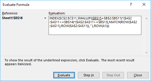
Press with left mouse button on "Evaluate" button, shown in above picture, to move to next step.
Step 1 - Compare value in cell B15 to cell range $B$2:$B$11
$B$15=$B$2:$B$11
returns {TRUE;FALSE;FALSE;... ;TRUE}
Step 2 - Compare start and end date to date column
($A$2:$A$11<=$B$14)*($A$2:$A$11>=$B$13)
returns {1;1;1;... ;0}
Step 3 - If a record is a match return it´s row number
IF(($B$15=$B$2:$B$11)*($A$2:$A$11<=$B$14)*($A$2:$A$11>=$B$13),MATCH(ROW($A$2:$A$11),ROW($A$2:$A$11))
returns {1;FALSE;FALSE;... ;FALSE}
Recommended articles
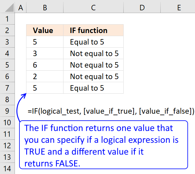
Checks if a logical expression is met. Returns a specific value if TRUE and another specific value if FALSE.
Step 4 - Return the k-th smallest value
SMALL(IF(($B$15=$B$2:$B$11)*($A$2:$A$11<=$B$14)*($A$2:$A$11>=$B$13),MATCH(ROW($A$2:$A$11),ROW($A$2:$A$11)),""),ROW(A1))
returns 1.
Recommended articles
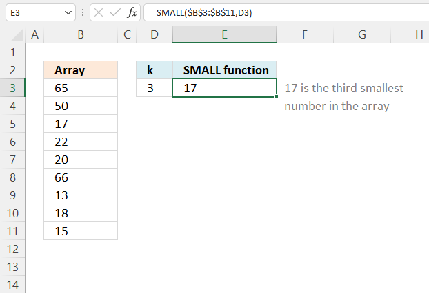
The SMALL function lets you extract a number in a cell range based on how small it is compared to the other numbers in the group.
Step 5 - Return the value of a cell at the intersection of a particular row and column
INDEX($C$2:$C$11,SMALL(IF(($B$15=$B$2:$B$11)*($A$2:$A$11<=$B$14)*($A$2:$A$11>=$B$13),MATCH(ROW($A$2:$A$11),ROW($A$2:$A$11)),""),ROW(A1)))
returns A in cell B18.
Recommended articles
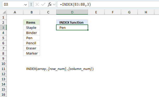
Gets a value in a specific cell range based on a row and column number.
4. Lookup a date range and a condition - return multiple values - Excel 365

Update: The new FILTER function is available for Excel 365 users. The regular formula in cell B18:
The FILTER function is a dynamic array formula meaning it returns an array of values to cell B18 and cells below automatically.
4.1 Explaining formula
Step 1 - Check which dates are larger or equal to the start date condition
The greater than and equal sign combined creates a logical test and the output is either True or False.
$B$3:$B$12>=$C$14
returns {TRUE; TRUE; TRUE; ... ; TRUE}.
Step 2 - Check which dates are smaller or equal to end date condition
$B$3:$B$12<=$C$15
returns {TRUE; TRUE; TRUE; ... ; FALSE}
Step 3 - Condition
$C$16=$C$3:$C$12
returns {TRUE; FALSE; FALSE; ... ; TRUE}
Step 4 - Multiply arrays - AND logic
The asterisk character multiplies the logical tests, this applies AND logic meaning:
TRUE * TRUE = TRUE
FALSE * TRUE = FALSE
TRUE * FALSE = FALSE
FALSE * FALSE = FALSE
($C$16=$C$3:$C$12)*($B$3:$B$12<=$C$15)*($B$3:$B$12>=$C$14)
returns {1; 0; 0; 0; 1; 0; 0; 0; 0; 0}.
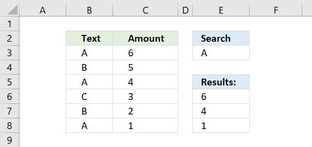
Step 5 - Filter values based on criteria
The FILTER function lets you extract values/rows based on a condition or criteria. It is in the Lookup and reference category and is only available to Excel 365 subscribers.
FILTER(D3:D12, ($C$16=$C$3:$C$12)*($B$3:$B$12<=$C$15)*($B$3:$B$12>=$C$14))
returns {"A";"E"}.
Index match category
This article demonstrates how to work with multiple criteria using INDEX and MATCH functions. Table of Contents INDEX MATCH - […]
Excel categories
39 Responses to “Lookup multiple values across columns and return a single value”
Leave a Reply
How to comment
How to add a formula to your comment
<code>Insert your formula here.</code>
Convert less than and larger than signs
Use html character entities instead of less than and larger than signs.
< becomes < and > becomes >
How to add VBA code to your comment
[vb 1="vbnet" language=","]
Put your VBA code here.
[/vb]
How to add a picture to your comment:
Upload picture to postimage.org or imgur
Paste image link to your comment.
ENTER IPC AET010AX
ACCT TYPE
Z.INP #N/A
Z.INPCDRHB #N/A
Z.INPCDTOX #N/A
Z.INPCDU #N/A
I want to be able to enter an IPC and have it come back with responsibility based on IPC and Acct type from the following table.
IPC SYSTEM ACCT TYPE RESPONSIBILITY
AET010AX CAMIS Z.INP Aetna
AET015AX CAMIS Z.INP Aetna Senior
AET015CC CAMIS Z.INP AETNA
BLC010AX CAMIS Z.INP Blue Cross
BLC015AX CAMIS Z.INP Blue Cross Senior
BLC015CC CAMIS Z.INP BLUE CROSS
BLC400CC CAMIS Z.INP BLUE CROSS
BLS010AX CAMIS Z.INP Blue Shield
I was using index with match with no luck. HELP
Candy,
Sheet2
Sheet1
Array formula in cell B4:
see attached file:
Candy.xlsx
i need to extract the headers from a grid based on value in left most column
example
row header ---> a b c d e
data 1 1 2 2 2
2 1 1
1 1 1 2
so how to find out which all headers appear agst 1 or 2o 3 in each row
vikas,
Read this post:
Match a criterion and extract multiple corresponding table headers
I have a worksheet(#1) and I want to populate the amount Column with data in another worksheet in the same workbook, Based on 2 criteria: State and Date
Worksheet #2 Table A1:D19 = EST
ColA ColB ColC ColD
1 AK 5/31 1st Installment 53,397.00
2 AK 8/31 2nd Installment 53,397.00
3 AK 11/30 3rd Installment -
4 AL 5/15 1st Installment -
5 AL 8/15 2nd Installment 53,349.00
6 AL 11/15 3rd Installment -
7 AR 5/15 1st Installment 33,237.00
8 AR 8/15 2nd Installment 33,237.18
9 AR 11/15 3rd Installment -
10 AZ 3/15 1st Installment 62,738.89
11 AZ 4/15 2nd Installment 62,738.89
12 AZ 5/15 3rd Installment 62,738.89
13 AZ 6/15 4th Installment 137,986.05
14 AZ 7/15 5th Installment 81,550.68
15 AZ 8/15 6th Installment 81,550.68
16 CA 4/1 1st Installment 495,364.00
17 CA 6/1 2nd Installment 495,364.00
18 CA 9/1 3rd Installment 495,364.00
19 CA 12/1 4th Installment -
Worksheet #1 I need the Worksheet 2 ColD amount to be put in the corresponding State and Date ColE on this worksheet. Can you help?
ColA ColB ColC ColD ColE
1 AK 5/31 -
2 AK 8/31 -
3 AK 11/30 -
4 AL 5/15 -
5 AL 8/15 -
6 AL 11/15 -
7 AZ 3/15 -
8 AZ 4/15 -
9 AZ 5/15 -
10 AZ 6/15 -
11 AZ 7/15 -
12 AZ 8/15 -
13 AR 5/15 -
14 AR 8/14 -
15 AR 11/14 -
16 CA 4/1 -
17 CA 6/1 -
18 CA 9/1 -
19 CA 12/1 -
Phoneix ,
read this: Fetch data from another table
Hi Oscar,
Thanks a lot.. for giving your time...
Can you please check the below file..
https://dl.dropbox.com/u/78831150/Excel/MultipleLookup.xlsm
* Which one is showing "Need to Overlook" they are VERIABLE..
* For each vendor I need to check his margin decider.. then according to margin Decider.. I need to LOOKUP.. correct Margin from Table 2..
Check attach file's Module.. for complete detail..
Apologize.. for increasing the confusion..
and requesting you to change the IMAGE (Lookup-multiple-conditions1.png) in post.. with latest one..
Regards,
Deb
Debraj,
Array formula in cell E2:
=INDEX($N$3:$N$11, MATCH(2, COUNTIF(A2, $J$3:$J$11)+COUNTIF(B2, $K$3:$K$11)+COUNTIF(C2, $L$3:$L$11)+COUNTIF(D2, $M$3:$M$11), 0))
Check this file:
MultipleLookup_solution.xlsm
Oscar..
amazing.. what an use of BINARY ADDITION..
Its always an eye pleasure to read your articles..
Thanks a ton...
Regards,
Deb
Hi Oscar,
One more silly question..
I tried to achieve the above by below formula..
=DGET(LookUpArea,"MARGIN",$P$2:$Q$3)
after Press F9 for $P$2:$Q$3 it gives me {"Vendor","Brick";"Chandoo","JEW"}
But if I set Criteria Array dynamic.. {"Vendor",E2;A2,Choose(Match,...)} it fails.. Is there any option to set ARRAY by Formula..
Regards,
=DEC2HEX(3563)
Debraj Roy,
Can you provide the array formula?
[...] shift enter NOT just enter, they can then be copied down. You may find some useful tips here.... Lookup multiple values in different columns and return a single value | Get Digital Help - Microsoft... Explaining a formula: Lookup values in a range using two or more criteria and return multiple [...]
VBA Code ?
Please help me with this I Need to look up several values and in the return the answer should be one.
Quantity On Hand Safety Stock Minimum Date
3/5/2013 7/5/2013 13/05/2013 21/05/2013 27/05/2013 30/05/2013
1.77 1.77 1.69 1.655 1.655 1.655 0.44
0 0 0 0 0 0 0
0 0 0 0 0 0 0
29.36 29.36 29.36 28.749 26.739 26.739 10
2.22 2.22 1.824 0.274 0.272 0.272 4.44
456.12 456.12 446.617 1086.769 1025.432 1025.432 850
8.766 8.766 8.029 8.029 8.029 8.029 15
Am,
Read this post:
Excel udf: Lookup and return multiple values concatenated into one cell
Hi Oscar,
I'm trying to utilize the formulas you've provided, but I'm unable to make them work with my data.
Essentially, I need Excel to bring back the value column C if the values match between column A and column D and column A-1 and column D-1.
A A-1 C D D-1 Column C Value
11:14 2037234 27600V 30 2000640
12:01 2016660 NL1000 "10" 2001931
30 2000640 060904 20,000 Years 2013724
42 2062442 201539 2001 2010036
187 2003556 097605 2010 2012514
300 2035604 200552 24 Hours to Kill 2001391
"10" 2001931 079813 36 Hours 2009741
Thanks in advance!
brett,
I am not sure which values you are looking for?
Blue values, array formula:
=INDEX($C$2:$C$8, SMALL(IF(COUNTIFS($A$2:$A$8, $D$2:$D$8, $B$2:$B$8,$E$2:$E$8)>0, MATCH(ROW($A$2:$A$8), ROW($A$2:$A$8)), ""), ROW(A1)),0)
Red values, array formula:
=INDEX($C$2:$C$8, SMALL(IF(COUNTIFS($D$2:$D$8,$A$2:$A$8, $E$2:$E$8,$B$2:$B$8)>0, MATCH(ROW($A$2:$A$8), ROW($A$2:$A$8)), ""), ROW(A1)), 0)
Get the Excel file:
Lookup-values-in-different-columns.xlsx
Thanks for looking into this Oscar! I'm looking to bring back values in column C only if there is a match in column A with column D, and a match in column B with column E.
I ended up figuring it out using this (array) formula:
INDEX($C$2:$C$6757,MATCH(1,IF($A$2:$A$6757=D2,IF($B$2:$B$6757=E2,1)),0))
As always, appreciate the help!
brett,
thank you for posting your solution.
Oscar, I thought, I was onto my solution with this but could not get it to play. So here's my problem. I'm trying to create a calendar tool, on sheet 1, I have column A with a list of days from jan-1 to dec-31. I have 10 users with assorted tasks on sheet 2. I am looking for a solution that will match the (Sheet 1)date row and the sheet 1 username from a drop down to all the matching row data on sheet 2. End result Example something like: sheet 1 populates the row "Dec 5 2013" with data from sheet 2 /B col user/ "Bob" /C col date/ Dec 5 2013 /f col task/ "Get Sleigh ready"/ z col/... and then.. Example: sheet 1 populates the row "Dec 12 2013" with sheet 2 /b user/ "Bob" /c col date/ Dec 5 2013 / f col task/ "Add rockets to Sleigh"/ z col/...
I'm sure for the wizard this is simple, but I'm out of ideas. Thank you kind sir!
Oscar,
INDEX('Tasks'!$F$6:$F$100,MATCH($A18,'Tasks'!$L$6:$L$29,0)) will work but I must delete all the other users from the second sheet. Or only works for one user. I would like to select the user name from a dropdown as a filter then apply the above index. Clueless.
thanks
Rae,
Oscar, I thought, I was onto my solution with this but could not get it to play. So here's my problem. I'm trying to create a calendar tool, on sheet 1, I have column A with a list of days from jan-1 to dec-31. I have 10 users with assorted tasks on sheet 2. I am looking for a solution that will match the (Sheet 1)date row and the sheet 1 username from a drop down to all the matching row data on sheet 2. End result Example something like: sheet 1 populates the row "Dec 5 2013" with data from sheet 2 /B col user/ "Bob" /C col date/ Dec 5 2013 /f col task/ "Get Sleigh ready"/ z col/... and then..
I understand this.
and then.. Example: sheet 1 populates the row "Dec 12 2013" with sheet 2 /b user/ "Bob" /c col date/ Dec 5 2013 / f col task/ "Add rockets to Sleigh"/ z col/...
I'm sure for the wizard this is simple, but I'm out of ideas. Thank you kind sir!
But not this? Why is row "Dec 12 2013" populated with values from date "Dec 5 2013"?
OK, Fresh look, that was careless, s/b same date. Basically at the top of sheet 1 column A is a dropdown of all my users below that has dates from jan1 to dec 31. In column b is the magical formula that matches the results of the dropdown "user" to the date in column A with like data on sheet 2.
sheet 1 Column C & D would be grabbing more of the row data from sheet 2 like Task, state, etc.
Does this make sense?
Rae,
Please upload an example file and I´ll see what I can do.
hi Oscar
in your response to Jason above under "Lookup multiple values in different columns and return multiple values" - i am also interested in returning and displaying a second column... so not only the Product A and E, but also the Product Price...
thus the results displayed should be:
Column B | Column C
A | $20
E | $10
I would like my customer to make a decision not just based on product but also on the price...
MR.OSCAR
THANKS FOR PROVIDING FOLLOWING FORMULA,BUT AFTER TWO VALUES FETCHED FOLLOWING CELL SHOWING NUM ERROR
=INDEX($C$2:$C$11, SMALL(IF(($B$15=$B$2:$B$11)*($A$2:$A$11=$B$13), MATCH(ROW($A$2:$A$11), ROW($A$2:$A$11)), ""), ROW(A1)))
IN ABOVE FORMULA IF I PUT A3 IN END OF FORMULA IT SHOWS NUM! I DO NOT WANT THIS PLEASE HELP ME IN THIS CASE,IF VALUE NOT MATCH TO FETCH THEN IT SHOULD BE SHOWN EMPTY CELL PLEASE DO THE NEEDFUL.
THANK YOU
REGARDS
SENTHILKUMAR
I have a tale as follows
date time open high low close
2-9 9:01:02 7500 7625 7500 7600
2-9 9:02:02 7600 7650 7600 7600
2-9 9:10:11 7600 7600 7550 7575
2-9 9:12:02 7575 7610 7530 7600
3-9 9:01:15 7600 7700 7600 7668
3-9 9:15:02 7668 7760 7500 7600
3-9 9:19:02 7600 7700 7500 7600
I need to look up a range for data to be arranged for a particular time range for a selected date. in the same format. how do I look up the 1st matching value as open for the time range of that date and also the high low between that date and time range and also the close
have a table as follows
date time open high low close
2-9 9:01:02 7500 7625 7500 7600
2-9 9:02:02 7600 7650 7600 7600
2-9 9:10:11 7600 7600 7550 7575
2-9 9:12:02 7575 7610 7530 7600
3-9 9:01:15 7600 7700 7600 7668
3-9 9:15:02 7668 7760 7500 7600
3-9 9:19:02 7600 7700 7500 7600
I need to look up a range for data to be arranged for a particular time range for a selected date. in the same format. how do I look up the 1st matching value as open for the time range of that date and also the high low between that date and time range and also the close
Hi Oscar,
I have sheet 1 and sheet 2. there r 4 columns in sheet 1 contains some values and sheet 2 having only one column. values are same in both sheet foe column a i want to extract the rest column details to sheet 2 from sheet 1. how can I ???
Hello Oscar,
I have 2 sheets, one that will have FP with different values and FO with different values. 2nd sheet will have the values to match to FP and FO. The problem that I am having is basically if value 1 and value 2 in FO, plus value 1 and value 2 in FP will result in the combination of those.
So, on sheet 2 is the array of values, example would be if on sheet 1, in the answer column, it would factor in the values of column A and column B based on the mapping in sheet 2.
Example, sheet 1, C1, Pipe, or sheet 1, C2,=Fla or sheet 1, C4,=Swi.
It can be set-up another way, but looking to take the value of two cell, if they match the mapping structure, then return the value on the far right. Thanks
Sheet 1
FP FO Answer
1 4
3 2
2 2
2 4
2 1
5 4
5 1
3 4
4 4
4 2
1 2
4 1
2 3
3 1
5 2
1 1
Sheet 2
FP1 FP2 FO1 FO2 Answer
1 2 1 3 Comm
3 4 1 2 Fla
1 2 2 Swi
3 4 4 Swi
Pipe
I have 30 questions in sheet2 and 20 questions in sheet3. so I want to get 10 question from sheet2 and 5 questions from sheet3 randomly. I want to question on sheet1 randomly. How can I get vba excell code it
hi Oscar
I have two columns(C1) and (C2) of integer values in Sheet1. I need a macro to search the values (c1) and (C2) and add it to sheet 2 (A1). The thing here is the columns (c1) and (c2) in sheet1 might exceed sometimes. So the macro should search the whole document sometimes. Please help
hi Oscar
I have two columns(C1) and (C2) of integer values in Sheet1. I need a macro to search the values (c1) and (C2) and add it to sheet 2 (A1). The thing here is the columns (c1) and (c2) in sheet1 might exceed sometimes. So the macro should search the whole document sometimes. Please help
Fab
Hi Oscar,
Please help.
1 6 A
2 5 B
3 4 C
4 3 D
5 2 E
6 1 F
i want my every cell of first column to search its value in column 2 and if it finds the value.....then it should copy the corresponding value of column 3 in column four corresponding to column1.
I means we have first column first cell as 1 and if it search it in column 2 it finds it in cell 6 and corresponding value to cell 6 is F....now it should paste this value F in column 4 but corresponding to column 1 cell 1
Hi Oscar, I need your help to solve my problem.. I have 2 columns in excel both with have values. If any one of the cell OR both cell contains "0" I need the output to be TRUE if not FALSE
VALUE1 VALUE2 OUTPUT
1234 7894 False
0 1234 TRUE
4567 0 TRUE
0 0 TRUE
-4567 0 TRUE
0 -984 TRUE
-7456 7456 FALSE
Thanks
Hii oscar
Help me to sort out it
I have
A1(anil singh raj)
It can be anything Like
A1(singh raj anil)
I want return value in
B1 (10 30 20)
Or
B1(30 20 10)
Or
Lookup array is
D1(anil) E1(10)
D2(raj) E2(20)
D3(singh) E3(30)
Kindly help me to do it?
I just wonder if the following two solutions might be preferable to your complex array entered formula:
Since you presented the data in an Excel table
1 by filtering the Date and Rep columns, you will find your answer within seconds, with no programming.
2 by using Get & Transform (Power Query), we can filter the entire table to return the results Jason wants:
#"Filtered Rows" = Table.SelectRows(#"Changed Type", each [Date] >= #date(2012, 1, 1) and [Date] <= #date(2012, 1, 6) and [Rep] = "John")
In both cases, changes to the start and end dates and to the Rep can be made very easily.
Duncan Williamson,
I just wonder if the following two solutions might be preferable to your complex array entered formula:
Yes, I know. You can also use an Excel defined Table.
This is a formula solution, this is sometimes useful in a dashboard or perhaps a dynamic chart.
Thank you for commenting.
Dear Oscar Cronquist,
Is it possible to change this Array formula in such way that is will not return the multiple values between two dates but that it returns the one value with the most recent date?
So in this example:
Search for: John
Result: J (as J is the one with the most recent date 2012-1-10)
Best regards,
Edu