INDEX MATCH – multiple results
This article demonstrates how to work with multiple criteria using INDEX and MATCH functions.
Table of Contents
- INDEX MATCH - multiple results
- INDEX and MATCH - multiple criteria and multiple results
- INDEX and MATCH - multiple criteria and multiple results (Excel 365)
- Get Excel *.xlsx file
- How to do a case sensitive INDEX MATCH - array formula
- How to do a case sensitive INDEX MATCH - regular formula
- How to do a case sensitive partial match using INDEX and MATCH functions
- How to do a partial case sensitive match using two conditions in two columns
- INDEX MATCH - multiple criteria
- INDEX MATCH - partial text multiple conditions Excel 365
- INDEX MATCH - partial match multiple columns
- INDEX MATCH - Last value
- Extract the last value in a given cell range
- Return a hyperlink to the last value in a column
- Return the row number of the last value in a column
- Extract a corresponding value next to the last value in a column
- Find the last non-empty cell with short cut keys
- Match two columns and return another value on the same row (array formula)
- Match two columns and return another value on the same row (regular formula)
- Match two columns and return another value on the same row - case sensitive
- Match two columns and return another value on the same row - partial match
- Get Excel *.xlsx file
- Find the closest value
- Find closest value - Excel 365
- Find closest values
- Find closest values and return adjacent values
- Find closest value with a criterion
1. INDEX and MATCH - multiple criteria and multiple results
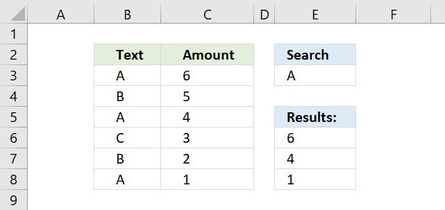
This section demonstrates how to use INDEX and MATCH functions to lookup and return multiple results. The lookup value is in cell E3, the lookup range is B3:B8.
Cells B3, B5, and B8 contains the lookup value, cell values in the corresponding cells in column C are returned. They are C3, C5, and C8.
There is actually a smaller formula that does the same thing: VLOOKUP - Return multiple values I also recommend the FILTER function if you are an Excel 365 user, the FILTER function is really easy to use.
The array formula in cell E6 extracts values from column C when the corresponding value in column B matches the value in cell E3.
The matching rows are 3, 5 and 8 so the array formula returns 3 values in cell range E6:E8.
The formula above is an array formula, make sure you follow the instructions below on how to enter an array formula to make it work.
1.1 How to enter an array formula
To enter an array formula, type the formula in a cell then press and hold CTRL + SHIFT simultaneously, now press Enter once. Release all keys.
The formula bar now shows the formula enclosed with curly brackets telling you that you entered the formula successfully. Don't enter the curly brackets yourself.
Now copy cell E6 and paste to cells below as far as needed.
1.2. Explaining formula in cell E6
Step 1 - Find matching values
The MATCH function matches a cell range against a single value returning an array.
MATCH($B$3:$B$8, $E$3, 0)
becomes
MATCH({"A"; "B"; "A"; "C"; "B"; "A"}, "A", 0)
and returns
{1; #N/A; 1; #N/A; #N/A; 1}.
If a value is equal to the search value MATCH function returns 1. If it is not equal the MATCH function returns #N/A.
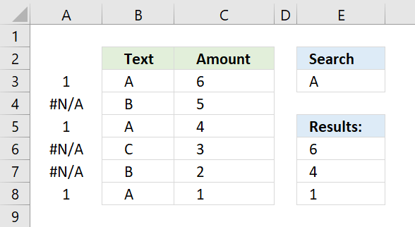
The picture above displays the array in column A.
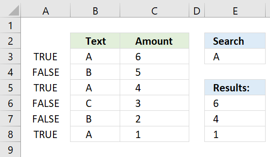
Step 2 - Convert array values to boolean values
The IF function cant process error values so to solve that I am going to use the ISNUMBER function to convert the array values to boolean values.
ISNUMBER(MATCH($B$3:$B$8, $E$3, 0))
becomes
ISNUMBER({1; #N/A; 1; #N/A; #N/A; 1})
and returns
{TRUE; FALSE; TRUE; FALSE; FALSE; TRUE}.
The array is shown in column A, see picture below.
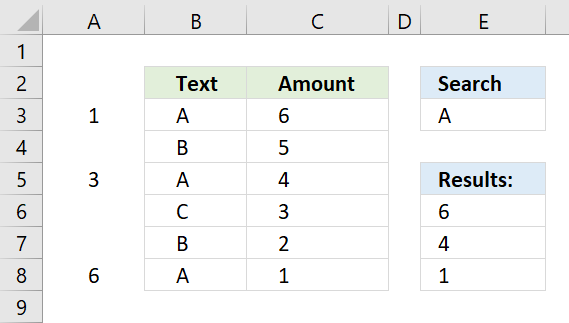
Step 3 - Identify rows
The IF function converts the boolean values into row numbers and blanks.
becomes
The MATCH and ROW functions calculate an array with sequential numbers, 1 to n, determined by the size of the cell range. In this case, $B$3:$B$8 has 6 values so the array becomes 1 to 6.
and returns
{1;"";3;"";"";6}.
The picture below shows the relative row numbers for cell range B3:B8.
Step 4 - Get the k-th smallest row number
To be able to return the correct value the formula must know which value to get. The SMALL function determines the value to get based on row number.
becomes
The ROWS function returns a number that changes when you copy the cell and paste to cells below.
and returns 1.
In the next cell below ROWS($A$1:A1) changes to ROWS($A$1:A2) and returns 2.
Step 5 - Get values from column C using row numbers
The INDEX function returns a value from a given cell range based on a row and column number.
becomes
The first cell value in cell range $C$3:$C$8 is 6, the INDEX function returns 6 in cell E6.
1.3. Get Excel file
2. INDEX and MATCH - multiple criteria and multiple results
This section demonstrates how to use INDEX and MATCH functions to match multiple conditions and return multiple results. The Excel 365 formula shown in section 2 is incredibly small, the new FILTER function is amazing.
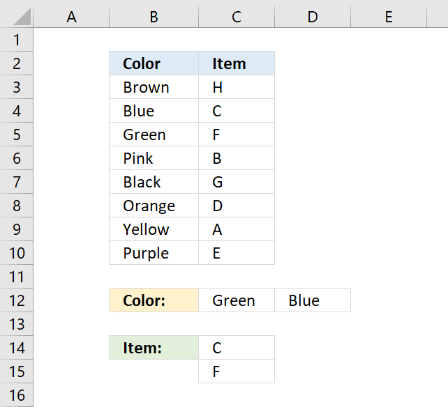
The formula in cell C14 returns multiple values from column Item. It uses multiple criteria specified in C12:C13 and applied to column Color.
This formula can only retrieve one value per criteria, read this article to extract multiple values per criteria.
This should be an array formula, however, the second INDEX function makes this formula a regular formula.
2.1 Explaining formula in cell C14
Step 1 - Find relative position of specified conditions in C12:D12
The MATCH function returns the relative position of an item in an array or cell reference that matches a specified value in a specific order.
MATCH(lookup_value, lookup_array, [match_type])
MATCH($C$12:$D$12, $B$3:$B$10, 0)
returns {3, 2}.
Step 2 - Get value based on the relative position
The INDEX function returns a value from a cell range, you specify which value based on a row and column number. However, in this case, it's used to convert the formula to a regular formula.
This is a workaround and it won't work in some array formula, it works fine in this one.
INDEX(array, [row_num], [column_num], [area_num])
INDEX(MATCH($C$12:$D$12, $B$3:$B$10, 0), )
returns {3, 2}.
Step 3 - Calculate k-th smallest number
The SMALL function returns the k-th smallest value from a group of numbers.
SMALL(array, k)
SMALL(INDEX(MATCH($C$12:$D$12, $B$3:$B$10, 0), ), ROWS($A$1:A1))
becomes
SMALL({3, 2}, ROWS($A$1:A1))
The ROWS function counts the number of rows in a given cell reference, however, $A$1:A1 is a cell reference that grows automatically when you copy the cell and paste it to cells below. This makes the formula return a new value in each cell.
SMALL({3, 2}, ROWS($A$1:A1))
returns 2.
Step 4 - Get value
The INDEX function returns a value from a cell range, you specify which value based on a row and column number. However, in this case, it's used to convert the formula to a regular formula.
This is a workaround and it won't work in some array formula, it works fine in this one.
INDEX(array, [row_num], [column_num], [area_num])
INDEX($C$3:$C$10, SMALL(INDEX(MATCH($C$12:$D$12, $B$3:$B$10, 0), ), ROWS($A$1:A1)))
returns "C" in cell C14.
3. INDEX and MATCH - multiple criteria and multiple results - Excel 365

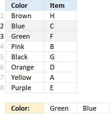
The new FILTER function is amazing, it returns multiple values based on boolean value TRUE or FALSE or their numerical equivalents.
Dynamic array formula in cell G3:
Excel 365 returns arrays automatically and deploys values to adjacent cells as far as needed, Microsoft calls this behavior "spilling".
Explaining formula in cell G3
Step 1 - Count values based on criteria
The COUNTIF function counts values based on a condition or criteria.
COUNTIF(range, criteria)
COUNTIF(E3:E4, B3:B10)
returns {0; 1; 1; 0; 0; 0; 0; 0}.
Step 2 - Get values
The FILTER function lets you extract values/rows based on a condition or criteria.
FILTER(array, include, [if_empty])
FILTER(C3:C10, COUNTIF(E3:E4, B3:B10))
returns {"C"; "F"}.
Get Excel *.xlsx file
INDEX and MATCH - multiple criteria and multiple results.xlsx
5. INDEX MATCH - Case sensitive
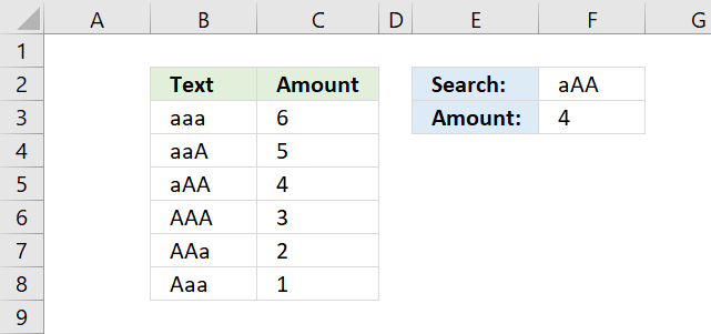
The picture above demonstrates a formula in cell F3 that allows you to look up a value in column B using the value in cell F2, also considering letter casing, then return the corresponding value from column C.
The image above shows text values in cells B3:B8 with different upper and lower case letters. Cell range C3:C8 contains the corresponding amounts. The formula in cell F3 performs a case sensitive search using the input value in cell F2 against the text values in B3:B8.
Formula in cell F3:
Cell F2 contains "aAA" and the formula returns 4 from the amounts in cells C3:C8. The formula matches "aAA" to cell value "aAA" in cell B5, the corresponding value in cells C3:C6 is 4.
How to enter an array formula
The formula above is an array formula. To enter an array formula, type the formula in a cell then press and hold CTRL + SHIFT simultaneously, now press Enter once. Release all keys.
The formula bar now shows the formula enclosed with curly brackets telling you that you entered the formula successfully. Don't enter the curly brackets yourself.
If you prefer a regular formula, read "Alternative regular formula" below in this section.
Explaining formula in cell F3
Step 1 - Compare lookup value with lookup column
The EXACT function allows you to compare values, if they are exactly the same the EXACT function returns TRUE. Note, the function is case-sensitive.
EXACT(F2,B3:B8)
becomes
EXACT("aAA",{"aaa"; "aaA"; "aAA"; "AAA"; "AAa"; "Aaa"})
and returns
{FALSE; FALSE; TRUE; FALSE; FALSE; FALSE}.
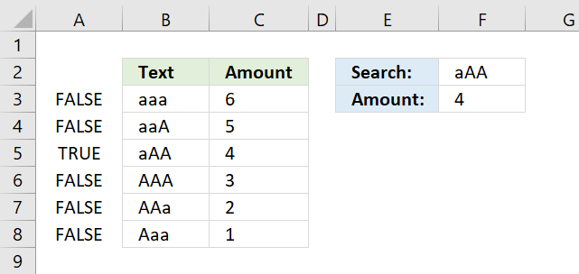
Step 2 - Identify the relative position of value TRUE in the array
The MATCH function finds a specific value in an array or cell range and returns its location, a number representing the position.
MATCH(TRUE,EXACT(F2,B3:B8),0)
becomes
MATCH(TRUE, {FALSE; FALSE; TRUE; FALSE; FALSE; FALSE}, 0)
and returns 3. TRUE is in the third position in the array.
Step 3 - Return corresponding value from column C
The INDEX function returns a value from an array or cell range based on the location. That is why the INDEX and MATCH functions work so well together.
INDEX(C3:C8,MATCH(TRUE,EXACT(F2,B3:B8),0))
becomes
INDEX(C3:C8,3)
becomes
INDEX({6;5;4;3;2;1},3)
and returns 4 in cell F3.
6. Alternative regular formula
Formula in cell F2:
7. How to do a case sensitive partial match using INDEX and MATCH functions

Formula in cell F3:
7. Explaining formula in cell F3
Step 1 - Perform a case sensitive search (partial match)
The FIND function returns a number representing the position of a specific substring in another string, reading left to right. Note, the FIND function is case-sensitive.
FIND(F2, B3:B8)
becomes
FIND("E", {"Cat"; "Horse"; "Snake"; "Tiger"; "Elephant"; "Mouse"})
and returns
{#VALUE!; #VALUE!; #VALUE!; #VALUE!; 1; #VALUE!}
Notice the error values in the array above, they appear if the substring is not found for each value in cell range B3:B8.
Step 2 - Identify numbers
The ISNUMBER function checks if a value is a number, it returns either TRUE or FALSE.
ISNUMBER(FIND(F2, B3:B8))
becomes
ISNUMBER({#VALUE!; #VALUE!; #VALUE!; #VALUE!; 1; #VALUE!})
and returns
{FALSE; FALSE; FALSE; FALSE; TRUE; FALSE}.
Step 3 - Find the position of the first number in the array
The MATCH function returns a number representing the relative position of an item in an array or cell reference that matches a specified value in a specific order.
MATCH(lookup_value, lookup_array, [match_type])
MATCH(TRUE, ISNUMBER(FIND(F2, B3:B8)), 0)
becomes
MATCH(TRUE, {FALSE; FALSE; FALSE; FALSE; TRUE; FALSE}, 0)
and returns 5. TRUE is first found in position five in the array above.
Step 4 - Get corresponding value from the same row
The INDEX function returns a value from a given cell range based on a row and column number (optional).
INDEX(array, [row_num], [column_num], [area_num])
INDEX(C3:C8, MATCH(TRUE, ISNUMBER(FIND(F2, B3:B8)), 0))
becomes
INDEX(C3:C8, 5)
becomes
INDEX({6;5;4;3;2;1}, 5)
and returns 2.
8. How to do a partial case sensitive match using two conditions in two columns

Formula in cell F3:
8.1 Explaining formula in cell F3
Step 1 - Perform a case sensitive search (partial match)
The FIND function returns a number representing the position of a specific substring in another string, reading left to right. Note, the FIND function is case-sensitive.
FIND(find_text,within_text, [start_num])
FIND(G4, B5:B10)
becomes
FIND("W", {"Brown"; "YeLLow"; "Pink"; "BLuE"; "BroWn"; "Black"})
and returns
{#VALUE!; #VALUE!; #VALUE!; #VALUE!; 4; #VALUE!}.
Step 2 - Perform a second case sensitive search (partial match)
FIND(G5, C5:C10)
becomes
FIND("M",{"small";"SMALL";"LaRgE";"SmAlL";"sMall";"small"})
and returns
{#VALUE!; 2; #VALUE!; #VALUE!; 2; #VALUE!}.
Step 3 - Multiply arrays
The formula returns a value if both substrings are found on the same row, to do that we need to apply AND logic.
The asterisk character lets you multiply values row by row, if both values are numbers the result is a number.
#VALUE! * #VALUE! = #VALUE!
#VALUE! * 2 = #VALUE!
2 * #VALUE! = #VALUE!
2*2 = 4
FIND(G4, B5:B10)*FIND(G5, C5:C10)
becomes
{#VALUE!; #VALUE!; #VALUE!; #VALUE!; 4; #VALUE!} * {#VALUE!; 2; #VALUE!; #VALUE!; 2; #VALUE!}
and returns
{#VALUE!; #VALUE!; #VALUE!; #VALUE!; 8; #VALUE!}.
Step 4 - Identify numbers
The ISNUMBER function checks if a value is a number, it returns either TRUE or FALSE.
ISNUMBER(FIND(G4, B5:B10)*FIND(G5, C5:C10))
becomes
ISNUMBER({#VALUE!; #VALUE!; #VALUE!; #VALUE!; 8; #VALUE!})
and returns {FALSE; FALSE; FALSE; FALSE; TRUE; FALSE}.
Step 5 - Find the position of the first number in the array
The MATCH function returns a number representing the relative position of an item in an array or cell reference that matches a specified value in a specific order.
MATCH(lookup_value, lookup_array, [match_type])
MATCH(TRUE, ISNUMBER(FIND(G4, B5:B10)*FIND(G5, C5:C10)), 0)
becomes
MATCH(TRUE, {FALSE; FALSE; FALSE; FALSE; TRUE; FALSE}, 0)
and returns 5.
Step 6 - Get corresponding value on the same row
The INDEX function returns a value from a given cell range based on a row and column number (optional).
INDEX(array, [row_num], [column_num], [area_num])
INDEX(D5:D10, MATCH(TRUE, ISNUMBER(FIND(G4, B5:B10)*FIND(G5, C5:C10)), 0))
becomes
INDEX(D5:D10, 5)
becomes
INDEX({1;2;3;4;5;6}, 5)
and returns 5.
8. Get Excel *.xlsx
INDEX MATCH Case sensitive.xlsx
9. INDEX MATCH with multiple criteria
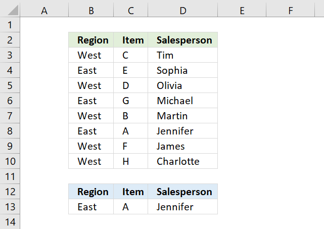
This section demonstrates formulas that let you perform lookups using two or more conditions. The image above shows two conditions in cells B13:C13, the result is in cell D13.
The formula in cell D13 returns the first match where both cells meet the conditions on the same row.
The formula demonstrated in cell D13 is a regular formula, most people prefer a regular formula over an array formula if possible, see the above picture.
The formula uses two conditions, one is specified in cell B13 and the other one in C13. It looks for the first condition in cell range B3 to B10 and the second condition in C3 to C10 if both conditions are met on the same row the corresponding name from cell range D3:D10 is returned.
9.1. Explaining formula in cell D13
Step 1 - Concatenate lookup values
The ampersand character concatenates both values you want to look for.
B13&C13
becomes
"East"&"A"
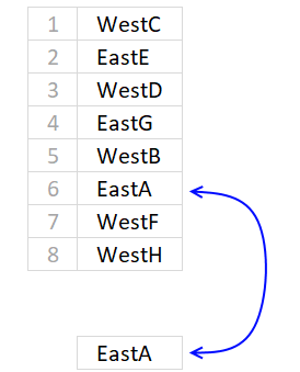
and returns "EastA".
Step 2 - Concatenate lookup columns
Then it concatenates the two cell ranges also using the ampersand character, the INDEX function makes it a regular formula.
B3:B10&C3:C10
returns {"WestC"; "EastE"; ... ; "WestH"}.
Step 3 - Make the array formula a regular formula
The INDEX function lets you convert some array formulas to regular formulas, this is one of them.
INDEX(B3:B10&C3:C10,)
The MATCH function then returns the relative position of the combined values, see picture above.
MATCH("EastA", {"WestC"; "EastE"; "WestD"; "EastG"; "WestB"; "EastA"; "WestF"; "WestH"}, 0)
and returns 6. The value is in the 6th position in the array.
Step 4 - Return value from the same row
INDEX(D3:D10, MATCH(B13&C13, INDEX(B3:B10&C3:C10, ), 0))
returns Jennifer in cell D13.
9.2 Array formula alternative
If you don't mind array formulas, the only advantage is that it is somewhat smaller, use this formula:
To enter an array formula press and hold CTRL + SHIFT simultaneously, then press Enter once. Release all keys.
The formula bar now shows the formula enclosed with curly brackets telling you that you entered the formula successfully. Don't enter the curly brackets yourself.
10. INDEX MATCH - partial text multiple conditions Excel 365

The formula in cell D13 checks if a cell in B3:B10 contains text specified in cell B13 and on the same row, if the corresponding cell in C3:C10 contains the specified text in C13.
The formula returns a value from D3:D10 if both cells are on the same row and contain the given text strings.
Excel 365 formula in cell D13:
=FILTER(D3:D10,ISNUMBER(SEARCH($B$13,$B$3:$B$10)*SEARCH($C$13,$C$3:$C$10)))
This is a dynamic array formula that works only in Excel 365, it is entered as a regular formula, however, it spills values to cells below if needed.
For previous Excel versions, see this article: Lookup with multiple criteria and return multiple search results It uses INDEX MATCH to get values based on multiple partial conditions.
10.1 Explaining formula in cell D13
Step 1 - Search for partial text in cell range B3:B10
The SEARCH function returns the number of the character at which a specific character or text string is found reading left to right (not case-sensitive)
SEARCH(find_text,within_text, [start_num])
This formula is copied to cells below in order to get all matching values. We need to use absolute references to lock cell ranges to prevent cell ranges from changing as we copy the cell and paste to cells below.
SEARCH($B$13,$B$3:$B$10)
returns {#VALUE!; #VALUE!; ... ; 4}.
Note that the SEARCH function returns a error value if the string is not found in a cell value.
Step 2 - Search for second partial text condition in cell range C3:C10
SEARCH($C$13, $C$3:$C$10)
returns {6; 4; ... ; #VALUE!}.
Step 3 - Multiply arrays
We will mutiply both arrays to perform AND logic by using the asterisk character.
SEARCH($B$13, $B$3:$B$10)*SEARCH($C$13, $C$3:$C$10))
returns {#VALUE!; #VALUE!; ... ; #VALUE!}.
A number multipled with an error value returns a error value, however, a number multipled with a number returns a number.
Step 4 - Check if a value in the array is a number
The ISNUMBER function returns TRUE or FALSE based on the contents of the argument.
ISNUMBER(SEARCH($B$13, $B$3:$B$10)*SEARCH($C$13, $C$3:$C$10))
returns {FALSE; FALSE;...; FALSE}.
Step 4 - Extract values based on logical array
The FILTER function returns values/rows based on a condition or criteria, it is only availabe to Excel 365 subscribers.
FILTER(D3:D10, ISNUMBER(SEARCH($B$13, $B$3:$B$10)*SEARCH($C$13, $C$3:$C$10)))
returns {"Olivia"; "Jennifer"}.
11. INDEX MATCH - partial match multiple columns

The array formula in cell D13 extracts values from column D if the corresponding value in cell range B3:C3 contains the specified string in cell B13.
The condition in cell B13 is found in cells B4, B6, and C8. The corresponding values in column D are in D4, D6, and D8.
Array formula in cell D13:
11.1 Explaining formula in cell D13
Step 1 - Search cell range $B$3:$C$10 for string
The SEARCH function returns the number of the character at which a specific character or text string is found reading left to right (not case-sensitive)
SEARCH(find_text,within_text, [start_num])
SEARCH($B$13, $B$3:$C$10)
returns {#VALUE!,#VALUE!;... ,#VALUE!}
Step 2 - Identify numbers in array
The ISNUMBER function returns TRUE or FALSE based on the contents of the argument.
ISNUMBER(SEARCH($B$13, $B$3:$C$10))*1
The MMULT function can't calculate boolean values like TRUE and FALSE, we need to convert them to their numerical equivalents. TRUE - 1 , and FALSE - 0 (zero)
returns {0,0; 1,0; 0,0; 1,0; 0,0; 0,1; 0,0; 0,0}.
Step 3 - Create an array containing 1
TRANSPOSE(COLUMN($B$3:$C$10)^0)
The COLUMN function returns row numbers based on a cell range.
COLUMN($B$3:$C$10)
returns {2,3}.
COLUMN($B$3:$C$10)^0
returns {1,1}.
TRANSPOSE(COLUMN($B$3:$C$10)^0)
becomes
TRANSPOSE({1, 1})
and returns {1; 1}.
Step 4 - Add values column-wise
The MMULT function calculates the matrix product of two arrays, an array as the same number of rows as array1 and columns as array2.
MMULT(array1, array2)
MMULT(ISNUMBER(SEARCH($B$13, $B$3:$C$10))*1, TRANSPOSE(COLUMN($B$3:$C$10)^0))
becomes
MMULT({0,0; 1,0; 0,0; 1,0; 0,0; 0,1; 0,0; 0,0}, {1; 1})
and returns {0; 1; 0; 1; 0; 1; 0; 0}.
Step 5 - Create an array from 1 to n
The ROW function lets you create numbers representing the rows based on a cell range.
The MATCH function finds the relative position of a given string in an array or cell range. This will create an array from 1 to n where n is the number of rows in cell range $D$3:$D$10.
MATCH(ROW($D$3:$D$10),ROW($D$3:$D$10))
and returns {1; 2; ... ; 8}. There are eight rows in $D$3:$D$10.
Step 6 - Replace 1 with corresponding row number
The IF function returns one value if the logical test is TRUE and another value if the logical test is FALSE.
IF(logical_test, [value_if_true], [value_if_false])
IF(MMULT(ISNUMBER(SEARCH($B$13, $B$3:$C$10))*1, TRANSPOSE(COLUMN($B$3:$C$10)^0)), MATCH(ROW($D$3:$D$10), ROW($D$3:$D$10)), "")
returns {""; 2; ""; 4; ""; 6; ""; ""}.
Step 7 - Extract k-th smallest row number
The SMALL function returns the k-th smallest value from a group of numbers.
SMALL(array, k)
SMALL(IF(MMULT(ISNUMBER(SEARCH($B$13, $B$3:$C$10))*1, TRANSPOSE(COLUMN($B$3:$C$10)^0)), MATCH(ROW($D$3:$D$10), ROW($D$3:$D$10)), ""), ROWS($A$1:A1))
becomes
SMALL({""; 2; ""; 4; ""; 6; ""; ""}, ROWS($A$1:A1))
becomes
SMALL({""; 2; ""; 4; ""; 6; ""; ""}, 1)
and returns 2.
Step 8 - Get values based on row number
The INDEX function returns a value from a cell range, you specify which value based on a row and column number.
INDEX($D$3:$D$10, SMALL(IF(MMULT(ISNUMBER(SEARCH($B$13, $B$3:$C$10))*1, TRANSPOSE(COLUMN($B$3:$C$10)^0)), MATCH(ROW($D$3:$D$10), ROW($D$3:$D$10)), ""), ROWS($A$1:A1)))
returns "Sophia".
The following formula is an Excel 365 dynamic array formula:
Absolute cell references are not required, the formula returns an array that spills values to cells below automatically.
11.4. Get Excel file
12. Find last value in a column

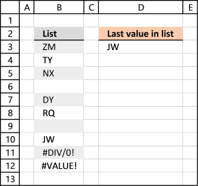
This section demonstrates formulas that return the last value in a given cell range or column. The image above shows a formula in cell D3 that extracts the last value from cell range B3:B12.
Cell range B3:B12 is populated with values and empty cells in random order, this shows that the formula works fine with empty cells.
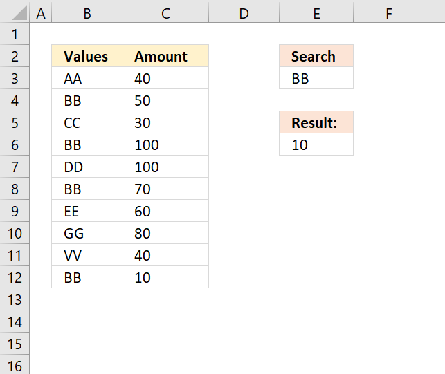
INDEX and MATCH are more versatile than the VLOOKUP function in terms of lookups, however, it only gets the first match. I have shown before how to lookup all matching values in this post: INDEX MATCH – multiple results and this article: VLOOKUP and return multiple values
Today I will show you how to get the last matching value, the image above demonstrates this formula in cell E6. It looks for value BB and the last matching value is found on row 12, the corresponding value in column C is 10 and this value is returned in cell E6.
Array formula in cell E6:
To enter an array formula, type the formula in a cell then press and hold CTRL + SHIFT simultaneously, now press Enter once. Release all keys.
The formula bar now shows the formula with a beginning and ending curly bracket telling you that you entered the formula successfully. Don't enter the curly brackets yourself.
Explaining formula in cell E6
Step 1 - Check if values are equal to lookup value
The equal sig lets you compare a cell value to another cell value, in this case, I am comparing a cell against an entire cell range.
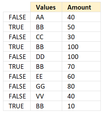 B3:B12=E3
returns {FALSE; TRUE; FALSE; ... ; TRUE}
Step 2 - Divide 1 with array
This step is special to the LOOKUP function, it allows us to get the last matching value.
1/(B3:B12=E3)
returns {#DIV/0!; 1; #DIV/0!;... ; 1}.
Step 3 - MATCH function
The MATCH function ignores error values and matches the last number smaller than the lookup value, in this specific situation.
MATCH(2,1/(B3:B12=E3)) returns 10.
Step 4 - INDEX function
The INDEX function returns a value from a cell range based on row an column numbers.
INDEX($C$3:$C$12,MATCH(2,1/(B3:B12=E3))) returns 10.
Get Excel *.xlsx file
13. Extract the last value in a given column

The formula in cell D3 lets you get the last value in column B, it works fine with blank cells in your list.
Formula in cell D3:
The formula is quite cpu-intensive since it is processing all cells in column B, there are more than a million cells in one column in Excel 2007 and later versions.
You can change the cell references if you know you will have a smaller list, this formula is easier for Excel to process:
13.1 Explaining formula
Then it divides 1 with the array creating errors for all empty cells.
The LOOKUP function ignores errors and tries to find a match. If every match is 1 and the lookup value is 2, the LOOKUP function returns last value in cell range. Normally the list must be sorted ascending for the LOOKUP function to work, however since every value is 1 there is no need to sort the list.
I am going to use the following formula because it will be easier to demonstrate:
LOOKUP(2,1/(B3:B12<>""),B3:B12)
Step 1 - Check if cells in column B are not equal to nothing
The less than and greater than signs are logical operators, they check if cell values in column B are not empty. The result is an array containing TRUE or FALSE.
B3:B12<>"" returns {TRUE;TRUE;TRUE; ... ;FALSE}
Step 2 - Divide 1 with array
1/(B3:B12<>"")
returns {1;1;1;... ;#DIV/0!}
Boolean value TRUE is equal to 1 and FALSE is equal to 0. You can't divide a value with zero so Excel returns an error (#DIV/0!).
Step 3 - Return value
LOOKUP(2,1/(B3:B12<>""),B3:B12) returns XH in cell D3.
13.2 What about errors?
I have added a few errors in column B, see the image above.
I am working with Excel 2016 and errors in column B seem to not be an issue.
14. Return a hyperlink to the last value in a column

The formula in cell D3, demonstrated in the image above, creates a hyperlink to the last cell in column B. Press with left mouse button on the hyperlink takes you to the last value in column B.
Formula in cell D3:
14.1 Explaining formula
Step 1 - Get path and workbook name
The CELL function gets information about the formatting, location, or the contents of a cell.
CELL("filename", A1)
returns C:\temp\[Find last value in listv2.xlsx]Hyperlink
Step 2 - Find the location of character [
We don't need the path in order to create a working hyperlink. This step returns the character of the first string that we do need.
The SEARCH function returns a number representing the position of character at which a specific text string is found reading left to right.
SEARCH("[", CELL("filename", A1)) becomes SEARCH("[", "C:\temp\[Find last value in listv2.xlsx]Hyperlink")
and returns 35.
Step 3 - Extract workbook and worksheet name
The MID function returns a substring from a string based on the starting position and the number of characters you want to extract.
MID(text, start_num, num_chars)
MID(CELL("filename", A1), SEARCH("[", CELL("filename", A1)), LEN(CELL("filename", A1)))
returns "[Find last value in listv2.xlsx]Hyperlink"
Step 4 - Concatenate workbook name, worksheet name, and column
The ampersand character & lets you concatenate strings in an Excel formula.
MID(CELL("filename", A1), SEARCH("[", CELL("filename", A1)), LEN(CELL("filename", A1)))&"!$B$"
returns "[Find last value in listv2.xlsx]Hyperlink!$B$".
Step 5 - Calculate row number of the last vale in a column
The ROW function allows you to calculate the row number of the last value.
MID(CELL("filename", A1), SEARCH("[", CELL("filename", A1)), LEN(CELL("filename", A1)))&"!$B$"&LOOKUP(2, 1/(B:B<>""), ROW(B:B))
returns "[Find last value in listv2.xlsx]Hyperlink!$B$11"
Step 6 - Return the last value
LOOKUP(2, 1/(B:B<>""), B:B)
returns "XH".
Step 7 - Create a hyperlink
The HYPERLINK function allows you to build a link in a cell pointing to something else like a file, workbook, cell, cell range, or webpage.
HYPERLINK(MID(CELL("filename", A1), SEARCH("[", CELL("filename", A1)), LEN(CELL("filename", A1)))&"!$B$"&LOOKUP(2, 1/(B:B<>""), ROW(B:B)), LOOKUP(2, 1/(B:B<>""), B:B))
returns a hyperlink to cell B11.
15. Return the row number of the last value in a column

The formula in cell D3 returns a number representing the row number of the last value in column B.
Formula in cell D3:
16. Return adjacent value
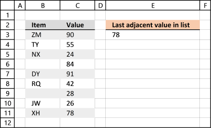
This data set has two columns B and C. The formula in cell E3 returns the corresponding value of the last value in column B from column C.
Formula in cell E3:
The formula returns an adjacent value of the last value. In fact, it doesn't need to be adjacent, you can change the cell reference (C:C) as long as its starting point and ending point are the same as the first cell reference (B:B).
17. Find the last non-empty cell with short cut keys

The following steps decribe how to select the last non-empty cell in column B using keyboard keys.
- Press with the left mouse button on cell A1 to select it.
- Press and hold CTRL key.
- Press down arrow key once. This takes you to the last cell in column A, if all cells in column A are empty.
- Release all keys. Press right arrow key to move to the last cell in column B.
- Press and hold CTRL key.
- Press up arrow key once. This takes you to the last non-empty cell in column B. See the image above.
18. Match two columns and return another value on the same row
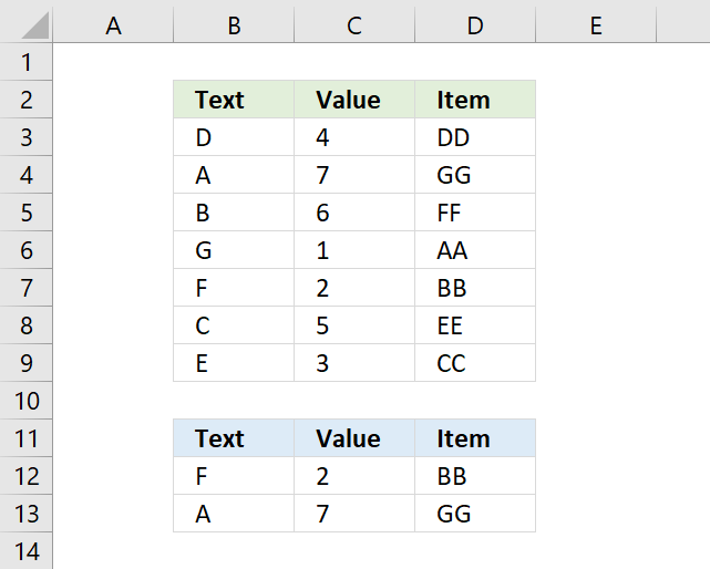
The array formula in cell D12 matches two values in two columns each and returns a value on the same row. First condition is specified in cell B12 and the second condition in cell C12.
The formula returns a value from cell range D3:D9 if both conditions are met on the same row. The example above returns cell value "NN" from cell D7.
Cell value "F" and "2" are found in cells B7 and C7, the corresponding value from cell D7 is returned to cell D12.
Formula in cell D12:
If you are looking for a way to compare two columns for differences or compare two columns for same values, please press with left mouse button on links.
You are not limited to formulas, conditional formatting allows you to compare two columns and highlight matches or compare two columns and highlight differences.
18.1 How to enter an array formula

To enter an array formula, type the formula in a cell then press and hold CTRL + SHIFT simultaneously, now press Enter once. Release all keys.
The formula bar now shows the formula enclosed with curly brackets telling you that you entered the formula successfully. Don't enter the curly brackets yourself.
Note that Excel 365 users can enter the formula as a regular formula.
18.2 Explaining formula
Step 1 - COUNT cells based on criteria
The COUNTIFS function counts rows where both values match, however, it returns an array that corresponds to the number of rows in cell range B3:D9.
COUNTIFS(B12, $B$3:$B$9, C12,$C$3:$C$9)
returns {0; 0; 0; 0; 1; 0; 0} , shown in column F in picture below.
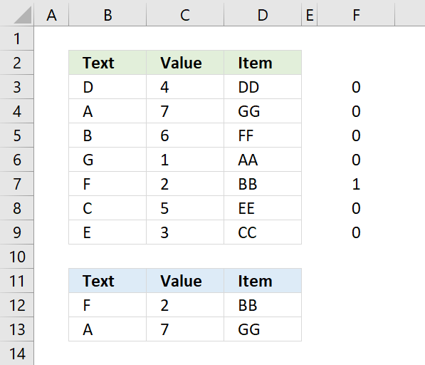
Both values match in row 7.
Step 2 - Calculate the relative position
The MATCH function returns a number representing the relative position of an item in an array or cell reference that matches a specified value in a specific order.
MATCH(lookup_value, lookup_array, [match_type])
MATCH(1, COUNTIFS(B12, $B$3:$B$9, C12,$C$3:$C$9) ,0)
The MATCH function identifies the relative position of the matching values.
MATCH(1, {0;0;0;0;1;0;0} ,0)
and returns 5, 1 is the fifth value in the array.
Step 3 - Get value
The INDEX function returns a value from a given cell range based on a row and column number (optional).
INDEX(array, [row_num], [column_num], [area_num])
INDEX($D$3:$D$9, MATCH(1, COUNTIFS(B12, $B$3:$B$9, C12,$C$3:$C$9) ,0))
The INDEX function returns the corresponding value from column D.
INDEX($D$3:$D$9, 5)
and returns BB in cell D12.
19. Match two columns and return another value on the same row - regular formula
This example is identical to the example above, however, it uses a regular formula mot an array formula.
Formula in cell D12:
The above formula is a regular formula, it is slightly larger than the first formula demonstrated above in section 1.
20. Match two columns and return another value on the same row - case sensitive

Formula in cell D12:
20.1 Explaining formula in cell D12
Step 1 - Identify values equal to value in cell B12 considering upper and lower case letters
The EXACT function lets you compare values also considering upper and lower cases.
EXACT(text1, text2)
EXACT(B12,$B$3:$B$9)
becomes
EXACT("F",{"D";"A";"f";"G";"F";"C";"a"})
and returns
{FALSE; FALSE; FALSE; FALSE; TRUE; FALSE; FALSE}.
Step 2 - Identify values equal to value in cell C12 considering upper and lower case letters
EXACT(C12,$C$3:$C$9)
becomes
EXACT(2, {4; 7; 2; 1; 2; 5; 7})
and returns
{FALSE; FALSE; TRUE; FALSE; TRUE; FALSE; FALSE}.
Step 3 - Multiply arrays AND logic
To apply AND logic we must multiply the arrays using the asterisk character.
EXACT(B12,$B$3:$B$9)*EXACT(C12,$C$3:$C$9)
becomes
{FALSE; FALSE; FALSE; FALSE; TRUE; FALSE; FALSE} * {FALSE; FALSE; TRUE; FALSE; TRUE; FALSE; FALSE}
and returns {0; 0; 0; 0; 1; 0; 0}.
Step 4 - Find position
The MATCH function returns the relative position of an item in an array or cell reference that matches a specified value in a specific order.
MATCH(lookup_value, lookup_array, [match_type])
MATCH(1, EXACT(B12,$B$3:$B$9)*EXACT(C12,$C$3:$C$9),0)
becomes
MATCH(1, {0; 0; 0; 0; 1; 0; 0},0)
and returns 5.
Step 5 - Get value based on row number
The INDEX function returns a value from a cell range, you specify which value based on a row and column number.
INDEX(array, [row_num], [column_num], [area_num])
INDEX($D$3:$D$9, MATCH(1, EXACT(B12,$B$3:$B$9)*EXACT(C12,$C$3:$C$9),0))
becomes
INDEX($D$3:$D$9, 5)
becomes
INDEX({"DD"; "GG"; "FF"; "AA"; "BB"; "EE"; "CC"}, 5)
and returns "BB" in cell D12.
21. Match two columns and return another value on the same row - partial match

Formula in cell D12:
21.1 Explaining formula in cell D12
Step 1 - Find position of first condition in string
The SEARCH function returns a number representing the position of character at which a specific text string is found reading left to right. The function is not doing a case-sensitive search.
SEARCH(find_text,within_text, [start_num])
SEARCH(B12, $B$3:$B$9)
becomes
SEARCH("esc",{"paper"; "investment"; "difference"; "mall"; "description"; "memory"; "judgment"})
and returns
{#VALUE!; #VALUE!; #VALUE!; #VALUE!; 2; #VALUE!; #VALUE!}
Notice the #VALUE! error, this is what you get if the string is not found.
Step 2 - Find position of the second condition in string
SEARCH(C12, $C$3:$C$9)
becomes
SEARCH("iet", {"supermarket"; "psychology"; "media"; "football"; "variety"; "difficulty"; "mud"})
and returns
{#VALUE!; #VALUE!; #VALUE!; #VALUE!; 4; #VALUE!; #VALUE!}.
Step 3 - Multiply arrays
Both arrays must return a number in the same position in the array, this can be created using the asterisk sign and multiplying the arrays.
SEARCH(B12, $B$3:$B$9)*SEARCH(C12, $C$3:$C$9)
becomes
{#VALUE!; #VALUE!; #VALUE!; #VALUE!; 2; #VALUE!; #VALUE!}* {#VALUE!; #VALUE!; #VALUE!; #VALUE!; 4; #VALUE!; #VALUE!}
and returns
{#VALUE!; #VALUE!; #VALUE!; #VALUE!; 8; #VALUE!; #VALUE!}.
Step 4 - Find the numbers in the array
The ISNUMBER function checks if a value is a number, returns TRUE or FALSE.
ISNUMBER(value)
ISNUMBER(SEARCH(B12, $B$3:$B$9)*SEARCH(C12, $C$3:$C$9))
becomes
ISNUMBER({#VALUE!; #VALUE!; #VALUE!; #VALUE!; 8; #VALUE!; #VALUE!})
and returns
{FALSE; FALSE; FALSE; FALSE; TRUE; FALSE; FALSE}.
Step 5 - Find the position of the first number in the array
The MATCH function returns the relative position of an item in an array or cell reference that matches a specified value in a specific order.
MATCH(lookup_value, lookup_array, [match_type])
MATCH(TRUE, ISNUMBER(SEARCH(B12, $B$3:$B$9)*SEARCH(C12, $C$3:$C$9)), 0)
becomes
MATCH(TRUE, {FALSE; FALSE; FALSE; FALSE; TRUE; FALSE; FALSE}, 0)
and returns 5. TRUE is the fifth value in the array.
Step 6 - Get value based on position
The INDEX function returns a value from a cell range, you specify which value based on a row and column number.
INDEX(array, [row_num], [column_num], [area_num])
INDEX($D$3:$D$9, MATCH(TRUE, ISNUMBER(SEARCH(B12, $B$3:$B$9)*SEARCH(C12, $C$3:$C$9)), 0))
becomes
INDEX($D$3:$D$9, 5)
and returns "BB". Value "BB" is the fifth value in D3:D9.
Get Excel *.xlsx
23. Find the closest value

The image above demonstrates a formula in cell E4 that extracts the closest number to the given number in cell E2.
Array formula in cell E4:
23.1 How to create an array formula
- Copy (Ctrl + c) and paste (Ctrl + v) array formula into formula bar.
- Press and hold Ctrl + Shift.
- Press Enter once
- Release all keys
23.2 Explaining array formula
Step 1 - Subtract numbers with search number
The minus sign lets you subtract numbers in an Excel formula.
B3:B25-E2
returns {-40; 34; ... ; 56}
Step 2 - Remove negative sign
The ABS function converts negative numbers to positive numbers.
ABS(number)
ABS(B3:B25-E2)
returns {40; 34; ... ; 56}
Step 3 - Find smallest number
The MIN function extracts the smallest number from in a cell range or array.
MIN(ABS(B3:B25-E2))
returns 1.
Step 4 - Find the relative position of the smallest number
The MATCH function returns the relative position of a given value in a cell range or array.
MATCH(lookup_value, lookup_array, [match_type])
MATCH(MIN(ABS(B3:B25-E2)),ABS(B3:B25-E2),0)
returns 12.
Step 5 - Get the number
The INDEX function returns a value based on a row and column number.
INDEX(array, row_num, [column_num])
INDEX(B3:B25,MATCH(MIN(ABS(B3:B25-E2)),ABS(B3:B25-E2),0))
returns 42.
24. Find closest value - Excel 365
Dynamic array formula in cell E4:
24.1 Explaining formula
Step 1 - Calculate the difference between numbers and search number
The minus sign allows you to subtract numbers in an Excel formula.
B3:B25-E2
becomes
{3; 77; 7; ... ; 99} - 43
and returns {-40; 34; ... ; 56}
Step 2 - Convert negative numbers to positive numbers
The ABS function converts negative numbers to positive numbers.
ABS(number)
ABS(B3:B25-E2)
returns {40; 34; ... ; 56}
Step 3 - Sort numbers based on difference
The SORTBY function allows you to sort values from a cell range or array based on a corresponding cell range or array. It sorts values by column but keeps rows.
It is located in the Lookup and reference category and is only available to Excel 365 subscribers.
SORTBY(array, by_array1, [sort_order1], [by_array2, sort_order2],…)
SORTBY(B3:B25, ABS(B3:B25-E2))
returns {42; 48; ... ; 99}
Step 4 - Get first value in array
The INDEX function returns a value from a cell range, you specify which value based on a row and column number.
INDEX(array, [row_num], [column_num], [area_num])
INDEX(SORTBY(B3:B25, ABS(B3:B25-E2)),1) returns 42 in cell E4.
25. How to find the closest values

The following array formula returns a list of numbers closest to the search number sorted from small to large.
Array formula in cell C4:
How to create an array formula
25.1 How to copy array formula
- Select cell C4
- Copy cell c4 (Ctrl + c)
- Select cell range C4:C20
- Paste (Ctrl + v)
25.2 Explaining formula
Step 1 - Subtract numbers with search number
The minus sign lets you subtract numbers in an Excel formula.
$A$2:$A$24-$E$1
returns {-40; 34; ... ; 56}.
Step 2 - Convert negative numbers to positive numbers
The ABS function converts any negative values to positive values.
ABS(number)
ABS($A$2:$A$24-$E$1)
returns {40; 34;... ; 56}
Step 3 - Extract the k-th smallest number
The SMALL function returns the k-th smallest number in a cell range or array.
SMALL(array, k)
The ROW function returns a number representing the row based on a cell reference.
ROW(ref)
SMALL(ABS($A$2:$A$24-$E$1), ROW(A1))
returns 1. Number 1 is the smallest number in the array.
Step 4 - Count based on condition
The COUNTIF function counts values based on a condition, in this case, a cell reference. Not a regular cell reference but an expanding cell reference that grows when you copy the cell to the cells below.
COUNTIF($C$3:C3, $A$2:$A$24)
returns {0; 0; ... ; 0}.
Step 5 - Count based on conditions
The COUNTIF function counts values based on a condition, in this case, based on multiple values.
COUNTIF($A$2:$A$24, $A$2:$A$24)
returns {1; 2; ... ; 1}.
Step 6 - Compare counts
The less than character lets you check if a value is smaller than another value, the result is a boolean value TRUE or FALSE.
COUNTIF($C$3:C3, $A$2:$A$24)<COUNTIF($A$2:$A$24, $A$2:$A$24)
returns {TRUE; TRUE; ... ; TRUE}.
Step 7 - Replace TRUE with corresponding positive number
The IF function returns one value if the logical test is TRUE and another value if the logical test is FALSE.
IF(logical_test, [value_if_true], [value_if_false])
IF(COUNTIF($C$3:C3, $A$2:$A$24)<COUNTIF($A$2:$A$24, $A$2:$A$24), ABS($A$2:$A$24-$E$1), "A")
returns {40; 34; ... ; 56}.
Step 8 - Calculate the relative position
The MATCH function returns the relative position of an item in an array or cell reference that matches a specified value in a specific order.
MATCH(lookup_value, lookup_array, [match_type])
MATCH(SMALL(ABS($A$2:$A$24-$E$1), ROW(A1)), IF(COUNTIF($C$3:C3, $A$2:$A$24)<COUNTIF($A$2:$A$24, $A$2:$A$24), ABS($A$2:$A$24-$E$1), "A"), 0)
returns 11. 1 is found in position 11 in the array or cell reference.
Step 9 - Get value
The INDEX function returns a value based on a row and column number.
INDEX(array, row_num, [column_num])
INDEX($A$2:$A$24, MATCH(SMALL(ABS($A$2:$A$24-$E$1), ROW(A1)), IF(COUNTIF($C$3:C3, $A$2:$A$24)<COUNTIF($A$2:$A$24, $A$2:$A$24), ABS($A$2:$A$24-$E$1), "A"), 0))
becomes
INDEX($A$2:$A$24, 11)
and returns 44.
Get excel file
26. How to find closest values and return adjacent values

Array formula in cell D5:
Array formula in cell E5:
How to create an array formula
26.1 How to copy array formula
- Select cell D5
- Copy (Ctrl + c)
- Select cell range D6:D28
- Paste (Ctrl + v)
27. Find closest value based on criterion
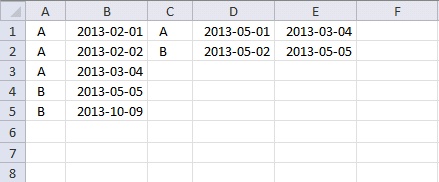
I need a formulae which will first match the entries in column A wih entries in column C .then compare the date in column D with the dates in column B and then throw up the nearest date.
So my data sheet looks something like this:
Col A Col B Col C Col D Col E(result)
A 1/2/2013 A 5/1/2013 4/3/2013
A 2/2/2013 B 5/2/2013 5/5/2013
A 4/3/2013
B 5/5/2013
B 9/10/2013
As you can see the formulae first compares the entries in col C (A) with the entries in col A (all the A's) then it matches the date in col D (5/1/2013) with the dates pertaining to value A in col B.
The closest date then is 4/3/2013 which is the answer.
Array formula in cell E1:
Workbook Find closest value
Workbook find closest value criterion
Index match category
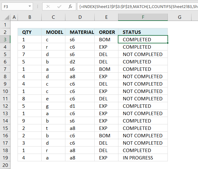
Table of Contents Lookup multiple values across columns and return a single value Lookup using multiple conditions Lookup a date […]
Excel categories
137 Responses to “INDEX MATCH – multiple results”
Leave a Reply
How to comment
How to add a formula to your comment
<code>Insert your formula here.</code>
Convert less than and larger than signs
Use html character entities instead of less than and larger than signs.
< becomes < and > becomes >
How to add VBA code to your comment
[vb 1="vbnet" language=","]
Put your VBA code here.
[/vb]
How to add a picture to your comment:
Upload picture to postimage.org or imgur
Paste image link to your comment.
looks like B.S. and does not work.
To prove that the formula works I have uploaded an excel workbook with the exact same values and formula as in this blog post.
Maybe you forgot to press CTRL + SHIFT + ENTER after you typed the formula?
It works, comment one needs to learn how to do their own work...
before calling BS on A CORRECT FORMULA.
Thank you for the help on this forumula this is exaclty what i was looking for
Could someone help me use this formula in German? Using excel in a different in language is kinda challenging =D
Translate excel functions from english to german: https://www.piuha.fi/excel-function-name-translation/index.php?page=deutsch-english.html
In the formula there are some colons (,) that should be semi-colons (;) if I am right;
--> =INDEX(A2:A26;MATCH(MIN(ABS(A2:A26-C1));ABS(A2:A26-C1);0))
hey,
I think that has to do with your regional settings. See this post: https://www.get-digital-help.com/excel-regional-settings/
Junk... Does not work
James,
Send me your excel file (without sensitive data) and I´ll see what I can do: https://www.get-digital-help.com/contact/
Hey, I don't know if this is specific to Excel 2010, however I found an error in your equation when attempting this in excel 2010, here is the corrected version of the equation:
=INDEX(D5:D36,MATCH(MIN(ABS(D5:D35-W8)),ABS(D5:D35-W8),0),0)
Ben Personick,
Your formula contains two different cell references, D5:D36 and D5:D35. What if the closest value is in cell D36?
hi oscar, i have a question that expands this topic ;)
above, there are 3 columns: [ID][OrderDate][Product].
search result would be in the columne where you put the formula in. <-- i call this [Result]
questions:
1) What if there are multiple columns? [ID][OrderDate][ProductA][ProductB][ProductC]?
this would output to [ResultA][ResultB][ResultC]
2) there are 3 methods above. I prefer Method 1 (plain 'ol formula only).
If I have 5000 (and growing) list of ID/OrderDates, which method would be practical?
thanks!
david,
1) You say you prefer the first formula:=INDEX(Product, SUMPRODUCT(--(C10=ID_num), --(C11=OrderDate), ROW(Product)-MIN(ROW(Product))+1)) + ENTER
I modified the above formula to get the other two matching cells:
=INDEX($D$3:$F$6, SUMPRODUCT(--($C$10=ID_num), --($C$11=OrderDate), ROW(ProductA)-MIN(ROW(ProductA))+1), COLUMN(A1)) + ENTER.
Copy cell and paste it to the right as far as needed.
Remember, this formula can only match one row. If multiple rows match you need another formula.
2) I think you answer your own question. If the first formula works and is reasonable fast, I´d also go with that one.
thx oscar, will try this out.
hi oscar,
i've tried the formula. it works but only if it's on the same sheet as the data.
if i move the formula on other sheet, it failed on the INDEX portion.
if u need a sample file, do let me know. i'll upload it somewhere for you :)
thanks!
assuming there is NO MATCH for ID and OrderDate ....by evaluating the formula when it's in INDEX portion, it gets
=INDEX($D$3:$F$6,0,1) <-- the row syntax=0 because there was no match.
however, it gets trickier.
if this formula is NOT within row 3-6, then it will generate an #VALUE error. (e.g. i put the formula at H8)
if i move this formula to a cell between row 3-6, the INDEX will pull the same value as per the row of the formula.
e.g. when the formula is at H4, the output is Green (D4). if formula at H5, the output is Yellow (D5).
so the question is, if there is NO MATCH for ID or OrderDate, how to output it as 0 (zero)?
thx :)
david,
Excel 2003:
=IF(SUMPRODUCT(--(C10=ID_num), --(C11=OrderDate), ROW(Product)-MIN(ROW(Product))+1)=0, 0, INDEX(Product, SUMPRODUCT(--(C10=ID_num), --(C11=OrderDate), ROW(Product)-MIN(ROW(Product))+1))) + Enter
Excel 2007:=IFERROR(INDEX(Product, SUMPRODUCT(--(C10=ID_num), --(C11=OrderDate), ROW(Product)-MIN(ROW(Product))+1)), 0) + Enter
hi oscar, thanks for your feedback.
i'm looking at Excel 2007 formula.
the IFERROR doesnt make any difference.
try this scenario:
1) move the B14 formula to H4
2) enter search ID = 4
3) u'll notice that it gives you the result as Green because the final formula step is =INDEX(Product,0,1) <-- the peculiarity occurs because the row syntax is 0.
Excel 2003's formula works though
david,
You are right, the excel 2007 formula is wrong.
Thanks!
Just a Typo. should have been D35 in each, D36 is blank.
Here it is using your original cell ranges instead:
=INDEX(A2:A26,MATCH(MIN(ABS(A2:A26-C1)),ABS(A2:A26-C1),0),0)
Hope that makes it clearer.
In excel 2010, an index can have two dimensions, and you must have a numerical value for both.
Ben Personick,
Thanks!
I want to find the two closest values (one above and one below) to my search value.
I would like a function that will perform this automatically as data is entered in to the search value cell.
The cntl+shift+enter is not a good solution for my spreadsheet. I need to see the results as the user enters the data and without any special key combinations.
Update.
Found two good solutions:
The first:
To find the closest larger number or an exact match in column A, use the SMALL and COUNTIF functions as shown in the following formula:
=SMALL($A$2:$A$7,COUNTIF($A$2:$A$7,"<"&B2)+1) To find the closest smaller number or an exact match in column A, use the LARGE and COUNTIF functions as shown in the following formula: =LARGE($A$2:$A$7,COUNTIF($A$2:$A$7,">"&B2)+1)
(https://www.exceltip.com/st/Retrieving_the_Closest_Larger_/_Closest_Smaller_Values_from_a_List_when_there_is_No_Exact_Match)/993.html)
It worked a treat, and then this solution from Eng-tips:
The second:
A1 is the search value. A2 to A11 the array and A12 and A13 the nearest values below and above:
In B1 put =MATCH(A1,A2:A11)
In A12 put =INDEX($A$2:$A$11,$B$1)
In A13 put =INDEX($A$2:$A$11,$B$1+1)
(https://eng-tips.com/viewthread.cfm?qid=280609&page=1)
To go one step further and choose the value closest to the search value is a simple IF statement:
{=IF((A1-A12)<(A13-A1),A12,A13)}
Note: The first of the two solutions works with unsorted data and the second using the MATCH function, with ordered data.
Hi,
The solution was veryvery helpful. Thanks for that!
However, facing a problem with decimal values.
I have a data say :: {C3:C5}{0.456,0.567,.678}
Data enterd in D1 cell : {0.560}
When trying to find out the closest value for it, the formula entered is :
=INDEX(C3:C5,MATCH(MIN(ABS(C3:C5-D1)),ABS(C3:C5-D1),0))
The value returned is always the first value from C3 i.e. 0.456.
Is there something i am missing out on???
Pradnya.Karmarkar,
I tried your example and the value returned here is 0,567. Maybe you forgot CTRL + SHIFT + ENTER?
Fantastic! Excellent Thank you
You are welcome!! Thanks for commenting!
Thanks, exactly what I needed
Hi,
Yes, now the example works. My cell given was wrong.
Thanks a lot !!!
Penny and Pradnya Karmarkar,
thanks for commenting!
Thanks for this.
Just in case others are as stupid as me:
It took me a while to figure out you need to press Ctrl SHIFT ENTER after typing (or pasting) the formula. Ctrl SHIFT ENTER is not part of the formula....
Stein,
Thanks!
I have edited this post and tried to explain how to create an array formula.
Thanks, this worked perfect after figuring out ctrl+shift+enter. Genious!
excellent tips. thanks for the help Oscar.
eben,
you are welcome!
Brilliant example - very many thanks.
Richard Moore,
Thank you for commenting!!
Excellent solution! Thanks a lot for this elegant tip...
Anurag,
Thanks!!
Excellent...
Thanks for sharing!
It did not work until I used CMD+SHIFT+ENTER (on a mac).
This looks like something I could use - I'm comparing two worksheets of school names and I need to get the closest match from to the other. Can this formula be altered to search in text strings? Thx
Hopefully, yes?
Jenna,
No, it can´t but maybe these blog posts can help you out:
https://www.get-digital-help.com/excel-udf-fuzzy-lookups/
https://www.get-digital-help.com/fuzzy-vlookup-excel-array-formula/
Hi,
I like the look of the formula and I have played around with the spreadsheet you updloaded but I cant get ABS to return multiple values. This is the problem I think people have been having. I have tried pasting your formula (ctrl+shift+enter) and rejig the cell references to suit my needs but I cant seem to get it to work. I worked through it with the evaluate function and the ABS function was returning a single value whereas with your it returns them all. How do I make it do this?
Anyone who is having trouble with this, research array formulas.
https://office.microsoft.com/en-us/excel-help/introducing-array-formulas-in-excel-HA001087290.aspx
There is a section that states you have to select all the cells that it applies to.
heath,
I have added a new section "How to find closest values" to this blog post. Check it out, I believe it answers your question.
execellent formula, thank you! i need some extra help though. i would like to return values corresponding to the nearest value.
For example, my data set is in column C and i returned the value nearest to what i was looking for; and found it to be in C6 for example. But i would also like to return the corresponding value in cell A6. Is there any way to do this?
Thanks again,
Cormac
Cormac,
read this: Find closest values and return adjacent values
THANK YOU VERY MUCH!
This really helps :-)
Awesome stuff, Oscar. Is there a way to use the version that returns the Adjacent Cell values with Excel 2003?
Thanks!
KK
KK,
No, I have no solution for you.
OK, thanks for the response.
I have a large array of numbers and a row of numbers. I want each number in the array to become higlighted one color if it is within 4 of any number in the row and another if it is not. Is this possible? Something like Abs(anynumber in array-any number in row < 4, Highlight green, highlight red) I think I have to utilize index or match functions but im having difficulty. Thanks!
Merit,
read post: Highlight values within specific ranges
thanks for sharing, I need help writing a formula that will return the closest higher (not less) value. thanks again
Agil,
just curious, why is an array formula needed here? I used a much simpler formula to acheive the same result. (unless i have missed something ofcourse.)
LOOKUP(E1,D:D,E:E)
This looks for the value in E1, finds the closest value or = to value in row D and returns the coorisponding value in row E.
Am i missing something that your formulas are doing?
Jeff :
For the LOOKUP function to work correctly, the data being looked up must be sorted in ascending order. If this is not possible, consider using the VLOOKUP, HLOOKUP, or MATCH functions.
And for the VLOOKUP and the HLOOKUP, the option range_lookup to find an approximate match needs the table_array to be placed in ascending sort order; otherwise, VLOOKUP might not return the correct value.
(Comes from Excel Help)
Jeff,
Sorry, I somehow forgot to answer your comment.
Jack is right,LOOKUP won´t work, even if you sort the values.
Let´s say you want to find the closest value to 43.
Values:
39
41
44
45
Lookup returns 41. 44 is closer to 43.
In the section "How to find closest values " . you said that the formula in C4 is
" =INDEX($A$2:$A$24, MATCH(SMALL(ABS($A$2:$A$24-$E$1), ROW(A1)), IF(COUNTIF($D$4:D4, $A$2:$A$24)<COUNTIF($A$2:$A$24, $A$2:$A$24), ABS($A$2:$A$24-$E$1), "A"), 0)) "
But, what is D4 refer to ?
And the function " COUNTIF " should have a condition after the set of values. while tou wrote " COUNTIF($A$2:$A$24, $A$2:$A$24) ". So, what is the condition ?
Simply you did a great work. But, i want to make the nearest value that appeared in C4 depend on a condition . If that condition is true, C4 will contain the closest value, if not, it will contain the next close value.
Thanks in advance
Amgad,
But, what is D4 refer to ?
You found an error, I have changed the formula.
And the function " COUNTIF " should have a condition after the set of values. while tou wrote " COUNTIF($A$2:$A$24, $A$2:$A$24) ". So, what is the condition ?
The countif function makes sure that the correct numbers are returned.
i want to make the nearest value that appeared in C4 depend on a condition . If that condition is true, C4 will contain the closest value, if not, it will contain the next close value.
See attached file:
find-closest-values-Amgad.xls
Took me forever trying to figure out why my formula wasn't working. All it took was CTRL+SHIFT+ENTER at the end of the formula in the formula bar. I never would have known that had I not found this site! Thanks Oscar!
Seth,
Thanks for commenting!
I have used the find closest values and it is working properly, but the find adjacent is not. I have gone over the formula mulitple times, but I cannot find an issue.
Find closest values - {=INDEX($E$3:$E$601,MATCH(SMALL(ABS($E$3:$E$601-$S$11),ROW(E1)),IF(COUNTIF($Z$2:Z2,$E$3:$E$601)<COUNTIF($E$3:$E$601,$E$3:$E$601),ABS($E$3:$E$601-$S$11),"A"),0))}
Find closest adjacent values - {=INDEX($A$3:$A$601,MIN(IF((Z3=$E$3:$E$601)*(COUNTIFS($Z$2:Z2,$E$3:$E$601,$V$2:V2,$A$3:$A$601)<COUNTIFS($E$3:$E$601,$E$3:$E$601,$A$3:$A$601,$A$3:$A$601)),MATCH(ROW($E$3:$E$601),ROW($E$3:$E$601)),"A")))}
Values in column E are the searched values, and column A is one of many adjacent values that I would like to display. Any help would be appreciated.
Edit* - I opened the sample spreadsheet and found that I am running an older version of excel that does not support the COUNTIFS function. I am not sure if I need to stack COUNTIF functions within a singular IF function to get the desired result or if there is a easier option?
Roland,
You are right, countifs does not work in 2003 and earlier versions.
This array formula works and it is in fact smaller than the excel 2007 version.
Array formula in cell E5:
Thanks for commenting!
Dear Oscar,
If I would like to use the closet number to choose number in the same row (instead of Text as your example). How can I write the formula?
Please guide me. I am really in beginner of using Excel formula.
Thank you for your help,
Note S
Note S,
I would like to use the closet number to choose number in the same row
can you explain in greater detail?
Hello OScar ,
I am trying to get a solution to find the 5 closest values . In the above example what if we have a multiple values in Column E . Could you please advise how to expand the scope .
Hari,
I am not sure I understand. Can you provide an example?
Hi Oscar, great job on the formula!
Just one question if you dont mind:
IN what corresponds to you A and B rows, I have something like that:
AAA 100
ABC 3
ABD 6
BBB 100
BCD 8
BDC 98
CCC 100
when i search the closest values and return adjacent values, i get it all right, except for the 100s. let say i search the closest values to 1, i would get, in the end of the list:
AAA 100
AAA 100
AAA 100
instead of AAA, BBB and CCC (whatever order).
Thanks in advance for your help,
S
SV,
I think you have the cell references wrong.
See attached file:
SV.xlsx
Thank you, you have taken 2 days of frustration away.
Alfredo,
Thank you for commenting!
Hi Oscar,
Great formula, very useful! I was just wondering, what would the formula look like if you want to search the closest value in a range of values in two columns? That is, in your example above, if the values were not in the range A2:A24 but in A2:B24. The formula doesn't work in that case as the index requires a row number and a column number. Any idea how to extend the formula so that is works on a larger range of values?
Many thanks!
Hi Oscar,
Is there a way to do this to find the closest value like in the first example but have excel return the closest number that is higher (even if it is not quite as close as another alternative that is lower than the value). I tried different websites for a solution to this and have had no luck. I'd really appreciate the help! Thanks.
Hi, I have a scenario where in I have different rates for may different product IDs which keeps on changing i.e. for a product I have several dates associated with rates. Now, I want to know the closest rate to a date per product. can you help me with that?
If you have two criteria to search
Cell C1 = value1
Cell C2 = value2
-the RESULT will be the index of A3:A30
-value2 will be located somewhere in a table B3:Q30
-you must first find the column(B3:Q3) of value1
-then using the column of value1, look for the closest match for value2 within that column
How would this formula be written?
Hi Oscar,
Require your help for finding the next closes negative and positive value based on the last value of the array.
Array (17 values)
=================
5182.47 4432.65 5285.95 3259.14 1731.73 1011.25 66.45 -203.18 -926.70 -1857.41 -3488.99 -4006.90 -4804.79 -5339.44 -6046.62 -6414.55 -6392.52
The last value is -6392.52, how do I get the next lowest (-6414.55) and the next highest (-6046.62) in relation to the last value of the array ? Please help.
Thanks,
S Srikanth
hi oscar,
I have this scenario, I have around 500 numeric values for example at column D, this values are composed of +/- value...then i sort it from lowest to largest...from this, if i have a reference number which is zero "0" how i can automatically select 200 closest value to my reference number? help appreciated....thanks
Hi Oscar,
How to get the closest value & it X and Y or may be in word (e.g. R3 & C6) in Table (2 Dimensional)?
E.g. of the Table, & the lookup value is 83
C1 C2 C3 C4 C5 C6
R1 03 66 82 34 12 87
R2 15 27 82 33 55 72
R3 29 53 57 32 65 44
R4 72 46 62 08 38 19
R5 26 99 44 97 80 78
R6 84 65 38 47 53 98
Thanks
CH
Hi,
so this is the case that I'm working on
XX 1/1/2016
XX 1/3/2016
XX 1/8/2016
YY 1/2/2016
YY 1/8/2016
ZZ 1/3/2016
ZZ 1/4/2016
ZZ 1/8/2016
So what I need is the closest or the same exact date
ex: XX 1/4/2016 -----> 1/3/2016 (out of 3 dates that has XX)
YY 1/8/2016 -----> 1/8/2016
ZZ 1/7/2016 -----> 1/8/2016
Thank you!
[…] https://www.get-digital-help.com/find-last-value-in-a-column/ […]
I'm building a workbook to search for any results that may use up to 34 criteria. So far I've built a formula from the website to fill six criteria, and I've hit a snag. The formula is creating duplicates. I want to avoid creating a list of results with duplicate values, then building a separate formula to create a list of unique values. Is there a way to do that all in one formula?
Here's the formula: =INDEX(Name,SMALL(IF(COUNTIF($E$20:$E$25,Category), MATCH(ROW(Category),ROW(Category)),""),ROWS($A$1:A1)))
Name = B3:B59
Category = AH3:AM59
Justin,
Yes, it is possible. If you enter the formula in cell F2 the formula becomes:
=INDEX(Name,SMALL(IF(COUNTIF($E$20:$E$25,Category)*(COUNTIF($F$1:F1,Category)=0), MATCH(ROW(Category),ROW(Category)),""),ROWS($A$1:A1)))
Any tips for doing this if theres multiple pairs of columns? Is it possible to concatenate results from multiple formulas of this kind into one column. For example lets say you were searching over 'n' pairs of the "text" and "amount" columns side by side, but still wanted the search results in a single column, like you have?
Joe Elizondo,
Yes, it is possible.
Array formula in cell C11:
=IFERROR(INDEX($C$3:$C$7, SMALL(IF(ISNUMBER(MATCH($B$3:$B$7, $C$9, 0)), MATCH(ROW($B$3:$B$7), ROW($B$3:$B$7)), ""), ROWS($A$1:A1))), INDEX($F$3:$F$7, SMALL(IF(ISNUMBER(MATCH($E$3:$E$7, $C$9, 0)), MATCH(ROW($E$3:$E$7), ROW($E$3:$E$7)), ""), ROWS($A$1:A1)-COUNTIF($B$3:$B$7, $C$9))))
The first formula didn't seem to work.
However, =INDEX(C3:C8, MATCH(TRUE, INDEX(EXACT(F2, B3:B8), ), 0))
worked for me.
Thank you :)
Sunil,
The first formula is an array formula. You probably didn't press CTRL + SHIFT + ENTER to create an array formula.
Assume, I have 3 column like A, B,c.and (D for using formula)
In column "A" there are some value between "B" and "c". and some are out of A- B range.
I need to fill the D column (if the value is between A and B and if not exist in A or B it takes value closest from A or closest from B
Hi Oscar,
This example helped me to get closer to what I am looking for, but not completely yet :).
In my case, I am looking to retrieve the sum of the results returned in a single cell.
First of all, I have converted your formula to column based:
The formula used is:
={IFERROR(INDEX($C$14:$L$14,SMALL(IF(ISNUMBER(MATCH($C$13:$L$13,C$16,0)),MATCH(COLUMN($C$13:$L$13),COLUMN($C$13:$L$13)),""),ROWS($A$1:A1))),0)}Text A G E C E A B G C C
Amount 2 4 1 3 2 3 1 3 1 2
Search A B C D E F G H
Results 2 1 3 0 1 0 4 0
3 0 1 0 2 0 3 0
0 0 2 0 0 0 0 0
0 0 0 0 0 0 0 0
0 0 0 0 0 0 0 0
0 0 0 0 0 0 0 0
0 0 0 0 0 0 0 0
0 0 0 0 0 0 0 0
SUM 5 1 6 0 3 0 7 0
As you see I have to create many rows to find all matches of each value. In my real case, I have more than 100 columns to match, and I don't know how many matches I will have. So I look for a way to return the sum of all matches (A - H) in a single row.
I am also working on a solution within VBA as back-up.
I hope you can help me. Please feel free to contact me if you need additional information.
Kind regards,
Jorgen
Hi Jorgen
Try this:
Formula in cell J3:
=SUMPRODUCT((B2:G13=I3)*1)
Hi Oscar,
This was super useful, thanks! I'm trying to take this one step further and be able to return all match instances of a certain value while having to search through more than a single-column array. To work through this using your example, I added a second column of Amounts and modified your formula to look up a given Amount and return the Text values that match that Amount. I got this to work with your INDEX(SMALL(IF(ISNUMBER(MATCH())))) and can pull all of the Text values from both Amount columns. I've also managed to return only Text values with that Amount from Amount2 using INDEX(MATCH(INDEX(MATCH))), however this can only find the first instance in the array. What I'm really trying to do is a combination of these: return all of the Text values within the given Amount array, while narrowing the search to a specific column within the array. Do you have any tips for this?
Formula in cell F5
=INDEX($B$2:$B$14, SMALL(IF(ISNUMBER(MATCH($C$2:$D$14, $F$2, 0)), MATCH(ROW($C$2:$D$14), ROW($C$2:$D$14)), ""), ROWS($A$1:A1)))Formula in cell G5
=INDEX($B$2:$B$14, MATCH($F$2, INDEX($C$2:$D$14, 0, MATCH($G$2, $C$1:$D$1,0)),0))Thanks,
Jeremiah
Jeremiah,
I believe you are looking for this formula:
https://www.get-digital-help.com/vlookup-a-range-in-excel/
Oscar,
Thanks for the reply. It looks like my image link didn't come through, trying again here:
https://imgur.com/a/FjajCCc
The article you referenced is close to what I'm looking for, but it doesn't allow me to narrow my search within the array to return all matches from only one desired column. Hopefully my example in the screenshot linked above will clarify this, the objective in cell H4 is what I'm trying to figure out a formula for.
Best,
Jeremiah
Jeremiah,
Formula in cell B14:
=INDEX($B$3:$B$6, SMALL(IF((INDEX($C$3:$E$6, 0, MATCH($C$10,$C$2:$E$2, 0))=$C$9)*(COUNTIF($B$13:B13, $B$3:$B$6)=0), ROW($C$3:$E$6)-MIN(ROW($C$3:$E$6))+1, ""), 1))
Hi Oscar,
Thank you very much for your article, it's very useful!
Regarding the last formula you've sent to Jeremiah, I'm also trying to have it working in a similar way but haven't been successful.
Basically instead of a match between a column and a row, I'm trying for the match of two columns to return the corresponding cells of a 3rd column.
Can you help me on this? Should I send what I have until now?
Best,
João
Table-1 Table-2
Number Name Number Name
10 A 10 search with Search result
11 B 13 C 13 #REF!
13 16 F
14 D 19 I
15 E 21 K
16
17 G
18 H
19
20 J
I have used this formula =+INDEX($D$3:$D12,MATCH($H4,$C$3:$C12,INDEX($G$3:$G7,MATCH($H4,$F$3:$F7,0))))
but is not working
I want there as 'C' because in Table-1 13 corresponding nothing so the formula should check with Table-2 with and result will be 'C'
Advance thanks
Hey Good Day,
can u do it if you have multiple person in same organization like
Org | Name | Badge | GC
649238 Rayn 64982 08
649238 Jhon 78421 11
649238 sara 76899 06
when i setup it with index match it gives me Rayn duplicated.
Rayn
The following link takes you to an article that demonstrates how to extract records based on a lookup value:
https://www.get-digital-help.com/how-to-return-multiple-values-using-vlookup-in-excel/#multiple
Thanks for the Tip, it already helped a lot, i just have the Problem, that my matches are not sorted from the earliest to the latest date. I don´t know why, because with the "SMALL" Funktion it should sort my matches by date beginning from the earliest date?
Flo
If column c contains dates that you want to extract based on a lookup value then use this array formula in cell E6:
=SMALL(IF($E$3=$B$3:$B$8, $C$3:$C$8, ""),ROWS($A$1:A1))
More examples here:
https://www.get-digital-help.com/small-function-and-large-function/
This article demonstrates how to use multiple conditions:
https://www.get-digital-help.com/small-function-multiple-criteria/
Oscar,
Your original set up almost answers my question, but I need to take it one step further. Instead of creating 3 rows in order to return the 6,4 & 1 values, I would like to sum all three into one cell. How do I do that.
https://i.postimg.cc/dVSffxhx/excell-1.jpg
https://i.postimg.cc/FHfpYsKT/excel2.jpg
So in my example, I would like to look up "B", and then lookunder the month of January, and sum up the number of "B"'s that is returned under that column. I just want the one row fo rth esum of B's. I dont want to have multiple cells that I still have to solve for, and I dont want to hid cells. Under the Cell for B, I might want to look up the Number of any letter in a particular month.
Does that make sense?
Thanks
Mike.
"Now copy cell E6 and paste to cells below as far as needed."
I would like to use data validation to allow the results to appear in a drop-down list in cell E6, instead of using the copy/paste instructions above. Is this possible?
Kyle
Yes, it is possible, however, you still need to extract the values using the formula perhaps on a different sheet.
I recommend a dynamic named range: Create a dynamic named range
Hello Oscar!
I'm new to excel and i just got employed in a firm that uses it a lot and im dealing with complex stuff so i really need some help.
I'm trying to make a table that will show me all the offers my employer made or is making by their status (i.e. in preparation, accepted, rejected etc).
This is the main table of offers https://imgur.com/1ilGTl0
What i need is: using the value in the right most column R(0-7) which shows the status of the offer, to get in,a new table, the left most column (column A) value (70-p/2019,72-p/2019) in an order without entering all that manually like im doin right now as shown in https://imgur.com/t8Kfp9N
I hope i was clear enough and that you can help me.
Looking forward to your response
Any idea why my formula is returning #N/A instead of the value I want? I am pretty sure it is working as intended because it should return 6 values and it is returning 6 #N/A and then #value. I am stumped. Is col A above a helper column? or is it all contained in the formula? Any assistance trouble shooting would be much appreciated!
Also, do you have any tips on how to write this for two variables? i.e return the corresponding customer if the variable is 5 or 6?
Adam,
Any idea why my formula is returning #N/A instead of the value I want?
Make sure the cell references are correct. You need to enter the formula as an array formula.
Is col A above a helper column?
No
or is it all contained in the formula?
Yes
Any assistance trouble shooting would be much appreciated!
I recommend you use "Evaluate Formula" tool found on tab "Formulas" on the ribbon.
Oscar, thanks so much! I really appreciate your assistance, the issue was the array formula, I overlooked that part in the initial article.
Thanks again!
what is wrong in this formula.
show #value
but in your excel sheet it shows correctly
=INDEX($L$2:$L$41,SMALL(IF(ISNUMBER(MATCH($M$2:$M$41,A2,0)),MATCH(ROW($M$2:$M$41),ROW($M$2:$M$41)),""),ROWS($A$1:A1)))
Thank you for publishing this wonderful guide. I am having one problem with it though. The formula returns the correct number of matches but each match listed is the first cell (cell O2) referenced in the index function. I need it to return the information matched for each cell from row 2.
=INDEX('[TUL_Heatmap_MES_All 2020.xlsm]2020'!$O$2:$BS$2,SMALL(IF(ISNUMBER(MATCH('[TUL_Heatmap_MES_All 2020.xlsm]2020'!$O$5:$BS$5,$B$7,0)),MATCH(ROW('[TUL_Heatmap_MES_All 2020.xlsm]2020'!$O$5:$BS$5),ROW('[TUL_Heatmap_MES_All 2020.xlsm]2020'!$O$5:$BS$5)),""),ROWS('[TUL_Heatmap_MES_All 2020.xlsm]2020'!$A$1:A1)))
May I ask How to Find the Last Match in a Range with a Wildcard? Thank you very much.
Grace,
Formula in cell E6:
=XLOOKUP(E3,B3:B12,C3:C12,"N/A",2,-1)
XLOOKUP is a new formula recently introduced to Excel 365 subscribers.
Grace,
Try this array formula if you own an earlier version of Excel.
=INDEX($C$3:$C$12,MATCH(2,1/SEARCH(E3,B3:B12)))
Dear Oscar
Thank you very much.
thanks again and again
Dear Oscar
Thank you very much.
thanks again and again
Guys how can I tell excel to ignore if the last match is NA?
Claudia,
(Array) formula in cell E6:
=INDEX($C$3:$C$12, MATCH(2, 1/((B3:B12=E3)*(NOT(ISNA(C3:C12))))))
Excel 365 subscribers do not need to enter the formula as an array formula.
Hi guys
How can I tell excel that I want second to last match as a result ???
This problem is difficult to explain, but I will try. I’m creating a database to keep track of stock option spread trades that have numerous legs. Some of the trades are simple and only having two legs, with one position being long, and the other being short. But, some of the trades have 8-10 legs, and this creates a problem in calculating the value of each leg. For this example, lets open a credit spread trade and go long an option, and go short an option. This is trade number 500 and each leg is recorded on a separate row. I want to invest $1000 per leg, so we need to take the ABS difference of the two fill prices and divide it $1000. This will tell us the quantity purchased. Eventually, we’ll close the short leg, and open a new short leg. And each time, we need to calculate a quantity by performing the above calculation with the long leg. This cycle of closing the short leg and opening a new short leg can continue until the long leg is finally closed, which ends the trade. So, let’s say we have 8-legs in this trade, the first row contains the long leg, and the 7 rows below contain the short legs. Each row has an ID of 500 to identify all 8-rows as trade number 500. Each time a short leg is closed, and a new short leg is opened, we need to scan the table for ID 500, then scan those rows to find the long leg. We then need to go over 5 columns to locate the long leg fill price to use in the new quantity calculation. Hope all that makes sense! Thanks, Jeff
Please can you explain why the MATCH lookup_value is 2?
Step3 example appears to repeat itself:
MATCH(2,{#DIV/0!; 1; #DIV/0!; 1; #DIV/0!; 1; #DIV/0!; #DIV/0!; #DIV/0!; 1})
becomes
MATCH(2,{#DIV/0!; 1; #DIV/0!; 1; #DIV/0!; 1; #DIV/0!; #DIV/0!; #DIV/0!; 1})
Penny's dropped, it's looking for the last number (1) smaller than the lookup value 2.
Maybe Step 3 should be:
MATCH(2,{#DIV/0!; 1; #DIV/0!; 1; #DIV/0!; 1; #DIV/0!; #DIV/0!; #DIV/0!; 1})
becomes
MATCH(2,{#DIV/0!; 1; #DIV/0!; 1; #DIV/0!; 1; #DIV/0!; #DIV/0!; #DIV/0!; 1},1)
Hi, I need to introduce a wildcard to this formula:
From this...
MATCH($B$3:$B$8, $E$3, 0)To this...
MATCH($B$3:$B$8, $E$3&"*", 0)But doing so breaks the formula. Do you have a workaround for this?
Hi Oscar, you are such a great resource. I was rocking right along until i copied the formula to the 12th column I received the #Num! error. Maybe I don't understand the ",ROWS($A$1:A1))),0)}" function. My data resides on two other sheets here is my formula:
=INDEX(STUDENT_A!$A$2:$A$6335, SMALL(IF(ISNUMBER(MATCH(STUDENT_A!$I$2:$I$6335, X$1, 0)), MATCH(ROW(STUDENT_A!$I$2:$I$6335), ROW(STUDENT_A!$I$2:$I$6335)), ""), ROWS(STUDENT_A!$A$1:$A1)))
Please advice. thanks
I got the exact same issue, also drawing from an external sheet. Any ideas?
Hello.
Thank you for publishing those awesome tutorials.
I am having a little problem here - I would like to test for the regular expression value (value you provided here in $E$3). It seems not to work.
I was trying to break the formulas to simple steps and everything seems to work fine if the value in the cell is exact match. Regular expressions seem to be treated as normal typing.
Do you know anything about it, maybe know a workaround?
Jakub
I believe you need VBA to be able to use regular expressions: https://www.get-digital-help.com/like-operator/
Hi Oscar,
Hoping you can help,
I'm trying to do an index and match multiple results across 2 groups with over 14,000 values to match.
I've tried to show an example below of what I'm trying to create.
I need to index a list of nested groups and users in sheet 1. Then match the group name they are a member of in sheet 2 with the same name in sheet 1 so that these values are pulled though to sheet 2 where the new group name is in a separate column.
DLG Domain 2 Returned Nested Groups`Users
DLG_1 Domain1\GG_Group
DLG_1 Domain2\GG_Group
DLG_1 User1
DLG_1 User2
DLG_2 Domain1\GG_Group
DLG_2 User1
DLG_2 User2
DLG_3 Domain1\GG_Group
DLG_3 Domain2\GG_Group
DLG_3 User1
DLG_3 User2
DLG_3 User3
Paul Quirie,
I think you are looking for this: https://www.get-digital-help.com/lookups-in-a-related-table-array-formula/
Dear Professor Oscar
I was wondering if there is a possibility, to simply ignore all text or blank cells and only search the maximum number value with the criteria in one column. It would also need the formula to be able to evaluate a cell which has mixed contents, like: "V20-001"
Here is the sample
Voucher criteria Result in Max Result in Min
V20-001 V20* V20-500 V20-001
X20-001 X20* X20-500 X20-001
V20-003
X20-100
V20-500
X20-500
X20-002
V20-002
I tried to use this formula:-=INDEX(A8:A51878,MATCH(2,1/SEARCH(A5,A8:A51878))) but it is not work.
Thank you very much.
Best regards,
Grace
Is there a way to ignore previous matched values? In the instance where there are multiple matches, that the formula will return the next matched value?
Many, many, many thanks! Exactly what I needed.
=you:you are great, TRUEI have app list with corresponding wave list. Each app can belong to multiple wave
Eg:
app1 Wave1
app1 Wave2
app2 Wave1
app1 Wave5
app1 Wave6
I am looking for result like this
app1 wave1, wave2, wave5, wave6...
The formula in this tutorial is to do multiple match function but i dont have definite wave number. each app can belong to 1 or 10 wave. its kind of like looping through wave and finding a match. so far I just have index & match function in 4 and more cells which is not very clean. any assitance appreciated. Thanks
Hi Oscar,
Thanks for this great article; it has helped me a lot!
Is there a way to pull multiple results from 12 different tables?
I have a table for each of the 12 months, and I need to pull specific data (based on a single criterion) from all 12 tables into one annual table.
I saw your reply to Joe regarding two different tables, but I couldn't figure out how to modify it for 12 different tables.
Any help is appreciated; thanks!
Hello sir
Can you please help me how to write this formula in vba with worksheet function?
=INDEX(A1:A26; MATCH(MIN(ABS(A1:A26-C1)); ABS(A1:A26-C1); 0))
Thank you