How to use the COLUMN function
What is the COLUMN function?
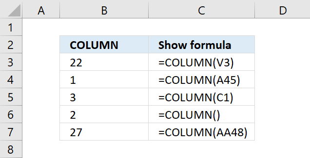
The COLUMN function returns the column number of the top-left cell of a cell reference. If the argument is not entered the column number of the cell the formula is entered in is returned, see cell B6 in the picture above.
Table of Contents
- Syntax
- Arguments
- Example
- How to convert a column number to a column letter?
- How to convert a column letter to a column number?
- How can the function return an array?
- VLOOKUP
- Other functions
- Cell ref to a cell range?
- Create a horizontal sequence
- SMALL function
- How to use the function in VBA
- Get Excel file
- Extract table headers based on a condition
- Function not working
1. Syntax
COLUMN(reference)
2. Arguments
| reference | Optional. The cell reference for which you want to extract the column number from. |
The COLUMN function allows you to also return an array of column numbers if you enter the formula as an array formula and use a cell range containing multiple columns.
You can not use multiple cell references in the COLUMN function.
3. Example
Formula in cell B3:
Column letter V corresponds to column number 22. A is 1, B is 2, and so on.
4. How to convert a column number to a column letter?

The formula in cell C3 calculates the column letter from a column number. Column number 1 is column A, column 2 is B, and so on. See the image above.
Formula in cell C3:
4.1 Explaining formula in cell C3
Step 1 - Calculate cell address
The ADDRESS function returns the address of a specific cell, you need to provide a row and column number.
ADDRESS(row_num, column_num, [abs_num], [a1], [sheet_text])
ADDRESS(1,B3,4,1)
becomes
ADDRESS(1,22,4,1)
and returns "V1".
Step 2 - Calculate number of characters in cell address
The LEN function calculates the number of characters in a given string.
LEN(ADDRESS(1,B3,4,1))-1
becomes
LEN("V1")-1
becomes
2-1 equals 1.
Step 3 - Extract column letter from cell address
The LEFT function extracts a specific number of characters always starting from the left.
LEFT(ADDRESS(1,B3,4,1), LEN(ADDRESS(1,B3,4,1))-1)
becomes
LEFT("V1", 1)
and returns "V" in cell C3.
5. How to convert a column letter to a column number?

The formula in cell C3 calculates the column number from a column letter. Column number 1 is column A, column 2 is B, and so on. See the image above.
Formula in cell C3:
5.1 Explaining formula in cell C3
Step 1 - Concatenate strings
The ampersand character lets you concatenate values.
B3&1
becomes
"V"&1
and returns "V1".
Step 2 - Create cell reference
The INDIRECT function returns the cell reference based on a text string.
INDIRECT(B3&1)
becomes
INDIRECT("V1")
and returns cell reference V1.
Step 3 - Calculate column number
COLUMN(INDIRECT(B3&1))
becomes
COLUMN(V1)
and returns 22 in cell C3.
6. How can the function return an array?

The COLUMN function calculates the column number from a cell reference, the column function returns an array of numbers if the cell reference points to a cell range that has multiple columns.
Formula in cell B3:
The formula in cell B3 returns a horizontal array of numbers from 1 to 3 representing the column numbers of cells A1, B1, and C1. Column letter A is 1, column 2 is B, and so on.
You need to enter this formula in cell B3 as an array formula if you own an earlier Excel version than Excel 365.
7. VLOOKUP

The formula in cell C3 combines the VLOOKUP and the COLUMN functions to get all values from the same row if the lookup value matches the leftmost value in the table array.
Formula in cell B3:
7.1 Explaining formula in cell C10
Step 1 - Calculate column number
The cell reference (B1) changes when you copy the cell and paste it to adjacent cells. This makes the COLUMN function return a different value in each cell.
COLUMN(B1) returns 2.
Step 2 - Evaluate VLOOKUP function
The VLOOKUP function lets you search the leftmost column for a value and return another value on the same row in a column you specify.
VLOOKUP(lookup_value, table_array, col_index_num, [range_lookup])
The third argument lets you choose which column to fetch a value from, this allows us to get all values from the same row when we copy the cell and paste it to adjacent cells.
VLOOKUP($B10,$B$3:$F$7,COLUMN(B1))
becomes
VLOOKUP($B10,$B$3:$F$7, 2)
and returns "ASD" in cell C10.
8. Other columns

The COLUMN function accepts no arguments at all, this will return the column number of the cell that the function is entered in.
Formula in cell B3:
The formula above does not change when you copy the cell and paste it to adjacent cells, however, the output is different. Cell C3 is the third column and therefore 3 is returned.
You can also use a cell reference to any other column or columns, see the formula below.
Formula in cell B6:
This formula returns the column number of cell K1 which is the argument used in this example. The cell reference is a relative cell reference meaning it changes when you copy the cell and pastes it to adjacent cells, see cell range C6:D6 in the image above.
The formula below returns an array of numbers 11, 12, and 13. They correspond to the cells in cell range K1:M1 and represent their column numbers.
Formula:
You need to enter this formula as an array formula in order to see all numbers in the array unless you are using Excel 365. Note that the array is a horizontal array with the same size as there are cells in the supplied cell range.
9. Cell ref to a cell range?

The COLUMN function repeats the array of numbers if entered in a cell range.
Array formula in cell B3:
Note, the formula is entered as a regular formula if your Excel version is 365.
10. Create a horizontal sequence

The COLUMN function can create a sequence of numbers that can be useful both in formulas and on a worksheet.
Formula in cell B3:
The formula above creates a horizontal sequence from 1 to n or as far as you copy the formula.
Formula in cell B6:
The formula in cell B6 creates a horizontal sequence containing odd numbers from 1 to n. Copy cell B6 and paste to adjacent cells on the same row as far as needed.
Formula in cell B9:
The formula in cell B9 creates a horizontal sequence containing odd numbers from 1 to n.
Note, relative cell references and the COLUMN function are sensitive to inserting rows and columns. The formula will break if you insert a column or row before the formula.
Use the COLUMNS function with a cell reference containing both an absolute and relative cell reference to solve this problem.
=COLUMNS($A$1:A1)
11. SMALL function

The COLUMN function combined with the SMALL function can extract and sort numbers from a cell range or array.
Formula in cell B8:
This is a regular formula.
11.1 Explaining formula in cell B8
Step 1 - Calculate sequence number
COLUMN(A1) returns 1.
Step 2 - Evaluate SMALL function
The SMALL function returns the k-th smallest value from a group of numbers. The first argument is a cell range or array that you want to find the k-th smallest number from.
The second and last argument is k which is a number from 1 up to the number of values you have in the first argument.
SMALL(array, k)
SMALL($B$3:$B$5, COLUMN(A1))
becomes
SMALL($B$3:$B$5, 1)
becomes
SMALL({5; -2; 3}, {1})
and returns -2.
12. How to use the COLUMN function in VBA?

The COLUMN function does not exist in the WorksheetFunction object. You can use the RANGE.COLUMN property to achieve the same thing.
The macro below saves the column number from cell B3 to cell B3. Column B is the second column.
Sub Macro1()

Range("B3") = Range("B3").Column

End Sub

14. Extract table headers based on a condition
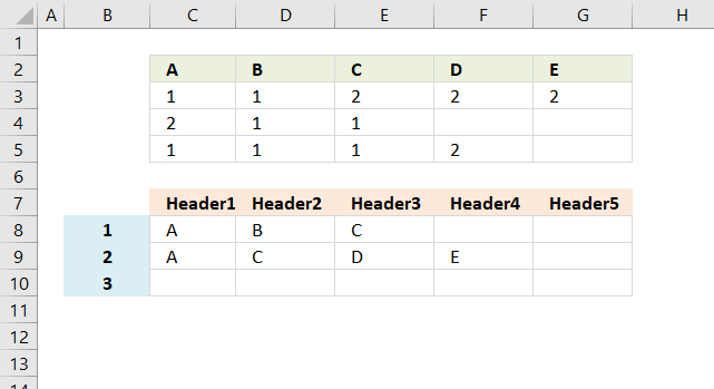
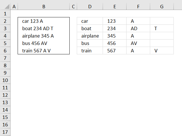
This article demonstrates an array formula that returns the table header based on a condition. For example, in cell C8 the formula returns A because 1 is found in cell C2 and C4.
The formula in cell C9 returns A because 2 is found once in cell range C3:C5, the condition is in column B.
i need to extract the headers from a grid based on value in left most column
example
row header ---> a b c d e
data 1 1 2 2 2
2 1 1
1 1 1 2
so how to find out which all headers appear agst 1 or 2o 3 in each row
The following array formula extracts column headers based on the condition in cell B8 and cells below.
Array formula in cell C8:
Excel 365 dynamic array formula in cell C8:
Copy cell C8 and paste to cells below as far as needed.
How to create an array formula
- Copy array formula
- Select cell B7
- Paste formula in formula bar
- Press and hold Ctrl + Shift
- Press Enter
How to copy array formula
- Select cell B7
- Copy cell (not formula)
- Select cell range C7:F7
- Paste (Ctrl +v)
Explaining array formula in cell C8
Step 1 - Filter column numbers
The IF function checks if value in cell B8 is equal to any of the cells in cell range C3:G5.
IF($B8=$C$3:$G$5, COLUMN($C$3:$G$5), "")
IF(logical_test, [value_if_true], [value_if_false])
The logical_test is $B8=$C$3:$G$5, it returns TRUE if equal and FALSE if not equal.
IF($B8=$C$3:$G$5, COLUMN($C$3:$G$5), "")
becomes
IF("1"={1, 1, 2, 2, 2;2, 1, 1, 0, 0;1, 1, 1, 2, 0}, {1, 2, 3, 4, 5}, "")
becomes
IF({TRUE, TRUE, FALSE, FALSE, FALSE;FALSE, TRUE, TRUE, FALSE, FALSE;TRUE, TRUE, TRUE, FALSE, FALSE}, {1, 2, 3, 4, 5}, "")
and returns
{1, 2, "", "", "";"", 2, 3, "", "";1, 2, 3, "", ""}
This array tells us that 1 is found in column 1, 2 and 3.
Step 2 - Calculate the frequencies of the numbers in the array
The FREQUENCY function allows you to extract only one instance of each header.
FREQUENCY(IF($B8=$C$3:$G$5, COLUMN($C$3:$G$5), ""), COLUMN($C$3:$G$5))
becomes
FREQUENCY({1, 2, "", "", "";"", 2, 3, "", "";1, 2, 3, "", ""}, {1, 2, 3, 4, 5})
and returns
{2;3;2;0;0;0}
If a value in this array is larger than 0 (zero) you know that the corresponding header is found in the cell range.
Step 3 - Extract unique distinct numbers
The IF function returns the corresponding column number if a value is larger than 0 (zero).
IF(FREQUENCY(IF($B8=$C$3:$G$5, COLUMN($C$3:$G$5), ""), COLUMN($C$3:$G$5))>0, ROW($A$1:$A$5), "")
becomes
IF({2;3;2;0;0;0}>0, {1; 2; 3; 4; 5}, "")
and returns
{1; 2; 3; ""; ""}
Step 4 - Return the k-th smallest value
The SMALL function returns the k-th smallest value in the array. SMALL(array, k)
SMALL(IF(FREQUENCY(IF($B8=$C$3:$G$5, COLUMN($C$3:$G$5), ""), COLUMN($C$3:$G$5))>0, MATCH(ROW($C$2:$C$6), ROW($C$2:$C$6)), ""), COLUMN(A1))
becomes
SMALL({1; 2; 3; ""; ""}, 1)
and returns 1.
Step 5 - Return the value of a cell at the intersection of a particular row and column
The INDEX function returns a value based on a row and column number.
INDEX($A$1:$E$1, SMALL(IF(FREQUENCY(IF($B8=$C$3:$G$5, COLUMN($C$3:$G$5), ""), COLUMN($C$3:$G$5))>0, MATCH(ROW($C$2:$C$6), ROW($C$2:$C$6)), ""), COLUMN(A1)))
becomes
INDEX($A$1:$E$1, 1)
becomes
INDEX({"A", "B", "C", "D", "E"}, 1)
and returns A in cell B7.
Step 6 - Return value_if_error if expression is an error and the value of the expression itself otherwise
The IFERROR function returns a blank (nothing) if an errror is returned.
=IFERROR(INDEX($A$1:$E$1, SMALL(IF(FREQUENCY(IF($B8=$C$3:$G$5, COLUMN($C$3:$G$5), ""), COLUMN($C$3:$G$5))>0, MATCH(ROW($C$2:$C$6), ROW($C$2:$C$6)), ""), COLUMN(A1))), "")
becomes
=IFERROR("A", "")
and returns A in cell C8.
15. Function not working
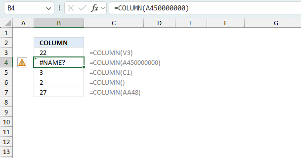
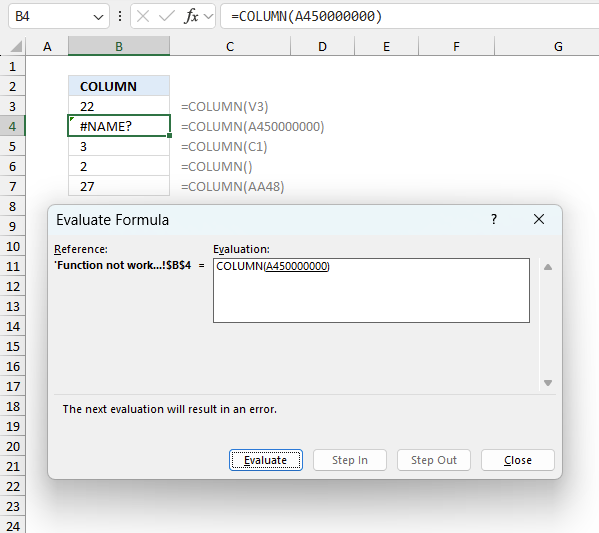
The COLUMN function returns a #NAME? error if you misspell the function name or if the cell reference is invalid.
15.1 Troubleshooting the error value
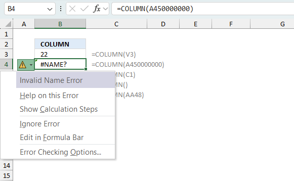
When you encounter an error value in a cell a warning symbol appears, displayed in the image above. Press with mouse on it to see a pop-up menu that lets you get more information about the error.
- The first line describes the error if you press with left mouse button on it.
- The second line opens a pane that explains the error in greater detail.
- The third line takes you to the "Evaluate Formula" tool, a dialog box appears allowing you to examine the formula in greater detail.
- This line lets you ignore the error value meaning the warning icon disappears, however, the error is still in the cell.
- The fifth line lets you edit the formula in the Formula bar.
- The sixth line opens the Excel settings so you can adjust the Error Checking Options.
Here are a few of the most common Excel errors you may encounter.
#NULL error - This error occurs most often if you by mistake use a space character in a formula where it shouldn't be. Excel interprets a space character as an intersection operator. If the ranges don't intersect an #NULL error is returned. The #NULL! error occurs when a formula attempts to calculate the intersection of two ranges that do not actually intersect. This can happen when the wrong range operator is used in the formula, or when the intersection operator (represented by a space character) is used between two ranges that do not overlap. To fix this error double check that the ranges referenced in the formula that use the intersection operator actually have cells in common.
#SPILL error - The #SPILL! error occurs only in version Excel 365 and is caused by a dynamic array being to large, meaning there are cells below and/or to the right that are not empty. This prevents the dynamic array formula expanding into new empty cells.
#DIV/0 error - This error happens if you try to divide a number by 0 (zero) or a value that equates to zero which is not possible mathematically.
#VALUE error - The #VALUE error occurs when a formula has a value that is of the wrong data type. Such as text where a number is expected or when dates are evaluated as text.
#REF error - The #REF error happens when a cell reference is invalid. This can happen if a cell is deleted that is referenced by a formula.
#NAME error - The #NAME error happens if you misspelled a function or a named range.
#NUM error - The #NUM error shows up when you try to use invalid numeric values in formulas, like square root of a negative number.
#N/A error - The #N/A error happens when a value is not available for a formula or found in a given cell range, for example in the VLOOKUP or MATCH functions.
#GETTING_DATA error - The #GETTING_DATA error shows while external sources are loading, this can indicate a delay in fetching the data or that the external source is unavailable right now.
15.2 The formula returns an unexpected value
To understand why a formula returns an unexpected value we need to examine the calculations steps in detail. Luckily, Excel has a tool that is really handy in these situations. Here is how to troubleshoot a formula:
- Select the cell containing the formula you want to examine in detail.
- Go to tab “Formulas” on the ribbon.
- Press with left mouse button on "Evaluate Formula" button. A dialog box appears.
The formula appears in a white field inside the dialog box. Underlined expressions are calculations being processed in the next step. The italicized expression is the most recent result. The buttons at the bottom of the dialog box allows you to evaluate the formula in smaller calculations which you control. - Press with left mouse button on the "Evaluate" button located at the bottom of the dialog box to process the underlined expression.
- Repeat pressing the "Evaluate" button until you have seen all calculations step by step. This allows you to examine the formula in greater detail and hopefully find the culprit.
- Press "Close" button to dismiss the dialog box.

There is also another way to debug formulas using the function key F9. F9 is especially useful if you have a feeling that a specific part of the formula is the issue, this makes it faster than the "Evaluate Formula" tool since you don't need to go through all calculations to find the issue.
- Enter Edit mode: Double-press with left mouse button on the cell or press F2 to enter Edit mode for the formula.
- Select part of the formula: Highlight the specific part of the formula you want to evaluate. You can select and evaluate any part of the formula that could work as a standalone formula.
- Press F9: This will calculate and display the result of just that selected portion.
- Evaluate step-by-step: You can select and evaluate different parts of the formula to see intermediate results.
- Check for errors: This allows you to pinpoint which part of a complex formula may be causing an error.
The image above shows cell reference A450000000 converted to hard-coded value using the F9 key. The COLUMN function requires valid cell references which is not the case in this example. We have found what is wrong with the formula.
Tips!
- View actual values: Selecting a cell reference and pressing F9 will show the actual values in those cells.
- Exit safely: Press Esc to exit Edit mode without changing the formula. Don't press Enter, as that would replace the formula part with the calculated value.
- Full recalculation: Pressing F9 outside of Edit mode will recalculate all formulas in the workbook.
Remember to be careful not to accidentally overwrite parts of your formula when using F9. Always exit with Esc rather than Enter to preserve the original formula. However, if you make a mistake overwriting the formula it is not the end of the world. You can “undo” the action by pressing keyboard shortcut keys CTRL + z or pressing the “Undo” button
15.3 Other errors
Floating-point arithmetic may give inaccurate results in Excel - Article
Floating-point errors are usually very small, often beyond the 15th decimal place, and in most cases don't affect calculations significantly.
'COLUMN' function examples

This post explains how to lookup a value and return multiple values. No array formula required.
This blog article describes how to split strings in a cell with space as a delimiting character, like Text to […]
In this blog post I will demonstrate methods on how to find, select, and deleting blank cells and errors. Why […]
Functions in 'Lookup and reference' category
The COLUMN function function is one of 25 functions in the 'Lookup and reference' category.
Excel function categories
Excel categories
5 Responses to “How to use the COLUMN function”
Leave a Reply
How to comment
How to add a formula to your comment
<code>Insert your formula here.</code>
Convert less than and larger than signs
Use html character entities instead of less than and larger than signs.
< becomes < and > becomes >
How to add VBA code to your comment
[vb 1="vbnet" language=","]
Put your VBA code here.
[/vb]
How to add a picture to your comment:
Upload picture to postimage.org or imgur
Paste image link to your comment.
Is it possible with2 criteria? with intersection table lookup?
Thans in advanced
Azumi
Azumi,
can you explain in greater detail`?
Something Like this (Intersection Tables:
A B C
AA 1 1 2
BB 2 1 2
How to retrieve column headers with this criteria:
1 and AA --> result should be A and B
or
1 and 2 and AA --> result should be A, B and C
Thanks
Hi Oscar, It helped me a great deal.
I was wondering if is it possible to count also how many times 1 exists in each header? please see the link for better understanding my query. Thanks!