How to list unique distinct values sorted by frequency

What's on this page
1. Unique distinct values sorted based on frequency (single column)
Array formula in D3:
copied down as far as needed.
How to create an array formula
- Copy above array formula
- Select cell D3
- Press with left mouse button on in formula bar
- Paste array formula in formula bar
- Press and hold Ctrl + Shift
- Press Enter
Formula in E3:
copied down as far as needed.
Explaining formula in cell D3
Step 1 - Calculate frequency of each value
The COUNTIF function counts values based on a condition, in this case, multiple conditions.
COUNTIF($B$3:$B$15, $B$3:$B$15)
becomes
COUNTIF({"DD"; "EE"; "GG"; "TT"; "EE"; "SS"; "YY"; "FF"; "GG"; "II"; "RR"; "TT"; "GG"}, {"DD"; "EE"; "GG"; "TT"; "EE"; "SS"; "YY"; "FF"; "GG"; "II"; "RR"; "TT"; "GG"})
and returns
{1; 2; 3; 2; 2; 1; 1; 1; 3; 1; 1; 2; 3}.
Step 2 - Prevent duplicate values
The first argument in the COUNTIF function contains an expanding cell reference. It makes sure that prior values are not taken into account again.
COUNTIF(D$2:$D2,$B$3:$B$15)<>1
becomes
COUNTIF("Unique distinct
list based on occurances", {"DD"; "EE"; "GG"; "TT"; "EE"; "SS"; "YY"; "FF"; "GG"; "II"; "RR"; "TT"; "GG"})<>1
becomes
{0;0;0;0;0;0;0;0;0;0;0;0;0}<>1
and returns
{TRUE; TRUE; TRUE; TRUE; TRUE; TRUE; TRUE; TRUE; TRUE; TRUE; TRUE; TRUE; TRUE}.
Step 3 - Multiply arrays
COUNTIF($B$3:$B$15, $B$3:$B$15)*(COUNTIF(D$2:$D2,$B$3:$B$15)<>1)
becomes
{1; 2; 3; 2; 2; 1; 1; 1; 3; 1; 1; 2; 3}* {TRUE; TRUE; TRUE; TRUE; TRUE; TRUE; TRUE; TRUE; TRUE; TRUE; TRUE; TRUE; TRUE}
and returns
{1;2;3;2;2;1;1;1;3;1;1;2;3}.
Step 4 - Check if largest value is equal to 0 (zero)
The IF function returns 1 if number is not equal to 0 (zero) and the largest value in array if equal to zero using the MAX function.
IF(MAX(COUNTIF($B$3:$B$15, $B$3:$B$15)*(COUNTIF(D$2:$D2, $B$3:$B$15)<>0))=0, 1, MAX(COUNTIF($B$3:$B$15, $B$3:$B$15)*(COUNTIF(D$2:$D2, $B$3:$B$15)<>1)))
becomes
IF(MAX({1;2;3;2;2;1;1;1;3;1;1;2;3})=0, 1, MAX(COUNTIF($B$3:$B$15, $B$3:$B$15)*(COUNTIF(D$2:$D2, $B$3:$B$15)<>1)))
becomes
IF(3=0, 1, MAX(COUNTIF($B$3:$B$15, $B$3:$B$15)*(COUNTIF(D$2:$D2, $B$3:$B$15)<>1)))
becomes
IF(FALSE, 1, MAX(COUNTIF($B$3:$B$15, $B$3:$B$15)*(COUNTIF(D$2:$D2, $B$3:$B$15)<>1)))
becomes
IF(FALSE, 1, 3)
and returns 3.
Step 5 - Find position in array
The MATCH function returns the position of a value in a cell range or array.
MATCH(IF(MAX(COUNTIF($B$3:$B$15, $B$3:$B$15)*(COUNTIF(D$2:$D2, $B$3:$B$15)<>0))=0, 1, MAX(COUNTIF($B$3:$B$15, $B$3:$B$15)*(COUNTIF(D$2:$D2, $B$3:$B$15)<>1))), COUNTIF($B$3:$B$15, $B$3:$B$15)*(COUNTIF(D$2:$D2, $B$3:$B$15)<>1), 0))
becomes
MATCH(3, COUNTIF($B$3:$B$15, $B$3:$B$15)*(COUNTIF(D$2:$D2, $B$3:$B$15)<>1), 0)
becomes
MATCH(3, COUNTIF($B$3:$B$15, $B$3:$B$15)*(COUNTIF(D$2:$D2, $B$3:$B$15)<>1), 0)
becomes
MATCH(3, {1;2;3;2;2;1;1;1;3;1;1;2;3}, 0)
and returns 3.
Step 6 - Return value
The INDEX function returns a value based on a row number (and column number if needed).
INDEX($B$3:$B$15, MATCH(IF(MAX(COUNTIF($B$3:$B$15, $B$3:$B$15)*COUNTIF(D$2:$D2,$B$3:$B$15)<>1)=0, 1, MAX(COUNTIF($B$3:$B$15, $B$3:$B$15)*IF(COUNTIF(D$2:$D2, $B$3:$B$15)=1,0,1))), COUNTIF($B$3:$B$15, $B$3:$B$15)*(COUNTIF(D$2:$D2, $B$3:$B$15)<>1), 0))
becomes
INDEX($B$3:$B$15, 3)
and returns "GG" in cell D3.
Get Excel *.xlsx file
Unique-distinct-list-sorted-based-on-occurrance-in-a-column-in-excel.xlsx
2. Unique distinct values sorted based on frequency - Excel 365

This formula works only with a single column cell range, read this article if you want to use a multi-column cell range: Extract a unique distinct list across multiple columns and rows sorted based on frequency
Excel 365 dynamic array formula in cell D3:
Explaining formula
Step 1 - Extract unique distinct values
The UNIQUE function extracts both unique and unique distinct values and also compare columns to columns or rows to rows.
UNIQUE(array,[by_col],[exactly_once])
UNIQUE(B3:B15)
becomes
UNIQUE({"DD"; "EE"; "GG"; "TT"; "EE"; "SS"; "YY"; "FF"; "GG"; "II"; "RR"; "TT"; "GG"})
and returns
{"DD"; "EE"; "GG"; "TT"; "SS"; "YY"; "FF"; "II"; "RR"}
Step 2 - Count values
The COUNTIF function calculates the number of cells that meet a given condition.
COUNTIF(range, criteria)
COUNTIF(B3:B15,UNIQUE(B3:B15))
Step 3 - Sort values based on count
The SORTBY function sorts values from a cell range or array based on a corresponding cell range or array.
SORTBY(array, by_array1, [sort_order1], [by_array2, sort_order2],…)
SORTBY(UNIQUE(B3:B15), COUNTIF(B3:B15,UNIQUE(B3:B15)),-1)
Step 4 - Shorten formula
The LET function lets you name intermediate calculation results which can shorten formulas considerably and improve performance.
LET(name1, name_value1, calculation_or_name2, [name_value2, calculation_or_name3...])
SORTBY(UNIQUE(B3:B15), COUNTIF(B3:B15,UNIQUE(B3:B15)),-1)
x - B3:B15
y - UNIQUE(x)
LET(x,B3:B15,y,UNIQUE(x),SORTBY(y,COUNTIF(x,y),-1))
3. Unique distinct values sorted based on frequency (multiple columns)
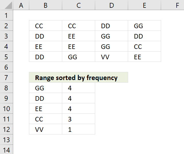
This array formula is for Excel versions prior to Excel 365, it works with a source containing multiple columns contrary to the first section above. The formula in cell B8 extracts a list sorted based on frequency based on cell range $B$2:$E$5.
Array formula in B8:
Enter the array formula in cell B8 the copy cell B8 and paste to cells below as far as necessary. I highly recommend the Excel 365 formula above, it so much smaller and easier to use.
Explaining formula in cell B8
Step 1 - Count previous values
The COUNTIF function counts values based on a condition or criteria. The first argument $B$7:B7 expands when the cell is copied to cells below.
COUNTIF($B$7:B7, tbl)=0
becomes
{0,0,0,0;0,0,0,0;0,0,0,0;0,0,0,0}=0
and returns
{TRUE, TRUE, TRUE, TRUE; TRUE, TRUE, TRUE, TRUE; TRUE, TRUE, TRUE, TRUE; TRUE, TRUE, TRUE, TRUE}
Step 2 - Replace TRUE with frequency count
The IF function returns the corresponding frequency number if boolean value is TRUE. FALSE returns "" (nothing).
IF(COUNTIF($B$7:B7,$B$2:$E$5)=0,COUNTIF($B$2:$E$5,$B$2:$E$5),"")
becomes
IF({TRUE, TRUE, TRUE, TRUE; TRUE, TRUE, TRUE, TRUE; TRUE, TRUE, TRUE, TRUE; TRUE, TRUE, TRUE, TRUE}, {3,3,4,4;4,4,4,4;4,4,4,3;4,4,1,4},"")
and returns
{3,3,4,4;4,4,4,4;4,4,4,3;4,4,1,4}.
Step 3 - Find largest value in array
The MAX function returns the maximum number in array ignoring blanks and text values.
MAX(IF(COUNTIF($B$7:B7, $B$2:$E$5)=0, COUNTIF($B$2:$E$5, $B$2:$E$5), ""))
becomes
MAX({3,3,4,4;4,4,4,4;4,4,4,3;4,4,1,4})
and returns 4.
Step 4 - Compare the largest number to array
IF((MAX(IF(COUNTIF($B$7:B7, $B$2:$E$5)=0, COUNTIF($B$2:$E$5, $B$2:$E$5), ""))=IF(COUNTIF($B$2:$E$5, $B$2:$E$5)*(COUNTIF($B$7:B7, $B$2:$E$5)=0), COUNTIF($B$2:$E$5, $B$2:$E$5)*(COUNTIF($B$7:B7, $B$2:$E$5)=0), "")), (ROW($B$2:$E$5)+(1/(COLUMN($B$2:$E$5)+1)))*1, "")
becomes
IF(4=IF(COUNTIF($B$2:$E$5, $B$2:$E$5)*(COUNTIF($B$7:B7, $B$2:$E$5)=0), COUNTIF($B$2:$E$5, $B$2:$E$5)*(COUNTIF($B$7:B7, $B$2:$E$5)=0), "")), (ROW($B$2:$E$5)+(1/(COLUMN($B$2:$E$5)+1)))*1, "")
becomes
IF(4={3,3,4,4;4,4,4,4;4,4,4,3;4,4,1,4}, (ROW($B$2:$E$5)+(1/(COLUMN($B$2:$E$5)+1)))*1, "")
becomes
IF(4={3,3,4,4;4,4,4,4;4,4,4,3;4,4,1,4}, {2.33333333333333, 2.25, 2.2, 2.16666666666667;3.33333333333333, 3.25, 3.2, 3.16666666666667;4.33333333333333, 4.25, 4.2, 4.16666666666667;5.33333333333333, 5.25, 5.2, 5.16666666666667}, "")
and returns
{"", "", 2.2, 2.16666666666667;3.33333333333333, 3.25, 3.2, 3.16666666666667;4.33333333333333, 4.25, 4.2, "";5.33333333333333, 5.25, "", 5.16666666666667}.
Step 5 - Replace TRUE with unique number
IF(MIN(IF((MAX(IF(COUNTIF($B$7:B7, $B$2:$E$5)=0, COUNTIF($B$2:$E$5, $B$2:$E$5), ""))=IF(COUNTIF($B$2:$E$5, $B$2:$E$5)*(COUNTIF($B$7:B7, $B$2:$E$5)=0), COUNTIF($B$2:$E$5, $B$2:$E$5)*(COUNTIF($B$7:B7, $B$2:$E$5)=0), "")), (ROW($B$2:$E$5)+(1/(COLUMN($B$2:$E$5)+1)))*1, ""))=(ROW($B$2:$E$5)+(1/(COLUMN($B$2:$E$5)+1))*1), $B$2:$E$5, "")
becomes
IF(MIN({"", "", 2.2, 2.16666666666667;3.33333333333333, 3.25, 3.2, 3.16666666666667;4.33333333333333, 4.25, 4.2, "";5.33333333333333, 5.25, "", 5.16666666666667})=(ROW($B$2:$E$5)+(1/(COLUMN($B$2:$E$5)+1))*1), $B$2:$E$5, "")
becomes
IF(2.16666666666667=(ROW($B$2:$E$5)+(1/(COLUMN($B$2:$E$5)+1))*1), $B$2:$E$5, "")
becomes
IF(2.16666666666667={2.33333333333333, 2.25, 2.2, 2.16666666666667;3.33333333333333, 3.25, 3.2, 3.16666666666667;4.33333333333333, 4.25, 4.2, 4.16666666666667;5.33333333333333, 5.25, 5.2, 5.16666666666667}, $B$2:$E$5, "")
becomes
IF({FALSE, FALSE, FALSE, TRUE; FALSE, FALSE, FALSE, FALSE; FALSE, FALSE, FALSE, FALSE; FALSE, FALSE, FALSE, FALSE}, $B$2:$E$5, "")
becomes
IF({FALSE, FALSE, FALSE, TRUE; FALSE, FALSE, FALSE, FALSE; FALSE, FALSE, FALSE, FALSE; FALSE, FALSE, FALSE, FALSE}, {"CC", "CC", "DD", "GG";"DD", "EE", "GG", "DD";"EE", "EE", "GG", "CC";"DD", "GG", "VV", "EE"}, "")
and returns
{"","","","GG";"","","","";"","","","";"","","",""}.
Step 6 - Concatenate strings in array
The TEXTJOIN function returns values concatenated ignoring blanks in array.
TEXTJOIN("", TRUE, IF(MIN(IF((MAX(IF(COUNTIF($B$7:B7, $B$2:$E$5)=0, COUNTIF($B$2:$E$5, $B$2:$E$5), ""))=IF(COUNTIF($B$2:$E$5, $B$2:$E$5)*(COUNTIF($B$7:B7, $B$2:$E$5)=0), COUNTIF($B$2:$E$5, $B$2:$E$5)*(COUNTIF($B$7:B7, $B$2:$E$5)=0), "")), (ROW($B$2:$E$5)+(1/(COLUMN($B$2:$E$5)+1)))*1, ""))=(ROW($B$2:$E$5)+(1/(COLUMN($B$2:$E$5)+1))*1), $B$2:$E$5, ""))
becomes
TEXTJOIN("", TRUE, {"","","","GG";"","","","";"","","","";"","","",""})
and returns "GG" in cell B8.
Get Excel *.xlsx file
Sort a range by frequency.xlsx
4. List unique distinct values sorted based on frequency (multiple columns) - Excel 365

This article demonstrates a formula that creates a frequency distribution table from a multi-column cell range which is useful in statistics.
The image above shows a cell range B2:E11 that contains values, the formula in cell B15 extracts unique distinct values in B2:E11, ignores blanks, and returns a list sorted based on frequency.
Dynamic array formula in cell B15:
Check out How to create a frequency table based on text values if your data is arranged in a single column.
Explaining formula
Step 1 - Rearrange values to a single column
The TOCOL function rearranges values in a 2D cell range to a single column.
TOCOL(array, [ignore], [scan_by_col])
TOCOL(B2:E11)
returns

Step 2 - Filter out blanks
The FILTER function extracts values/rows based on a condition or criteria.
FILTER(array, include, [if_empty])
FILTER(TOCOL(B2:E11), TOCOL(B2:E11)<>"")
returns

The empty cells are now gone in cell B13 and cells below.
Step 3 - Extract unique values
The UNIQUE function extracts both unique and unique distinct values and also compare columns to columns or rows to rows.
UNIQUE(array,[by_col],[exactly_once])
UNIQUE(FILTER(TOCOL(B2:E11), TOCOL(B2:E11)<>""))
returns
{"Banana"; "Lime"; "Pineapple"; "Strawberry"; "Orange"; "Pear"; "Raspberry"; "Apple"}.

Step 4 - Count values
The COUNTIF function calculates the number of cells that meet a given condition.
COUNTIF(range, criteria)
COUNTIF(B2:E11, UNIQUE(FILTER(TOCOL(B2:E11), TOCOL(B2:E11)<>"")))
becomes
COUNTIF(B2:E11, {"Banana"; "Lime"; "Pineapple"; "Strawberry"; "Orange"; "Pear"; "Raspberry"; "Apple"})
and returns
{6; 3; 6; 4; 4; 3; 3; 5}.
Step 5 - Sort values based on the frequency
The SORTBY function sorts values from a cell range or array based on a corresponding cell range or array.
SORTBY(array, by_array1, [sort_order1], [by_array2, sort_order2],…)
SORTBY(UNIQUE(FILTER(TOCOL(B2:E11), TOCOL(B2:E11)<>"")), COUNTIF(B2:E11, UNIQUE(FILTER(TOCOL(B2:E11), TOCOL(B2:E11)<>""))), -1)
becomes
SORTBY({"Banana"; "Lime"; "Pineapple"; "Strawberry"; "Orange"; "Pear"; "Raspberry"; "Apple"}, {6; 3; 6; 4; 4; 3; 3; 5}, -1)
and returns
{"Banana"; "Pineapple"; "Apple"; "Strawberry"; "Orange"; "Lime"; "Pear"; "Raspberry"}.
Step 6 - Shorten the formula
The LET function lets you name intermediate calculation results which can shorten formulas considerably and improve performance.
LET(name1, name_value1, calculation_or_name2, [name_value2, calculation_or_name3...])
SORTBY(UNIQUE(FILTER(TOCOL(B2:E11), TOCOL(B2:E11)<>"")), COUNTIF(B2:E11, UNIQUE(FILTER(TOCOL(B2:E11), TOCOL(B2:E11)<>""))), -1)
x - B2:E11
y - TOCOL(x)
z - UNIQUE(FILTER(y,y<>""))
LET(x,B2:E11,y,TOCOL(x),z,UNIQUE(FILTER(y,y<>"")),SORTBY(z, COUNTIF(x,z),-1))
Useful resources
How to make a frequency distribution table in Excel - pivot table
How to Make a Histogram in Excel (Step-by-Step Guide)
Frequency table category
More than 1300 Excel formulasExcel categories
14 Responses to “How to list unique distinct values sorted by frequency”
Leave a Reply
How to comment
How to add a formula to your comment
<code>Insert your formula here.</code>
Convert less than and larger than signs
Use html character entities instead of less than and larger than signs.
< becomes < and > becomes >
How to add VBA code to your comment
[vb 1="vbnet" language=","]
Put your VBA code here.
[/vb]
How to add a picture to your comment:
Upload picture to postimage.org or imgur
Paste image link to your comment.
Your array formulas are very interesting.
But this fails if there is two or more values whith the same frequency.
Many thanks and best regards
Thanks for your comment! I have changed the formula and the attached excel file. The formula doesn´t work with blank cells.
Hi, very nice formula! I´m trying to do something like this, but I need to show one more column at the side of each unique element with the count of occurrences :-)
Fernando,
In the above example, try this formula in C9 copied down as far as necessary.
=COUNTIF(tbl, B9) + CTRL + SHIFT + ENTER
How can we do that in Excel 2010? without VBA or PowerTools or PowerPivot etc. but only using worksheet formulas. I can do it in VBA. I am asking because it's very hard to figure out using only worksheet formulas. Thanks in advance. Since dates were not shown, I would like to record my request as made on 07MAY2023.
T S,
This article will probably show you how: Unique distinct values sorted based on frequency if you can rearrange your values to a single column.
Hi, the formula given is missing a pair of parentheses thus returning only UNIQUE values not UNIQUE and DISTINCT values.
But your explanation on calculation steps contains the correct formula.
Thank you for sharing this formula.
https://i.imgur.com/fgxAyKd.png
T S,
thank you for telling me. I hope I got it right now.
Hi, I took the liberty of editing the formula presented here into one that does not require CSE.
I did it because most beginners have trouble pressing that key combo.
My editition might affect performance but if it's a very large data set (column), I don't think much will be affected on most modern computers.
I think the basic principle is still the same as the one already shared here.
=IF(SUMPRODUCT(1*(COUNTIF(T$2:$T2, $B$3:$B$12)=0))=0,"",INDEX($B$3:$B$12,MATCH(AGGREGATE(14,6,COUNTIF($B$3:$B$12, $B$3:$B$12)*(COUNTIF(T$2:$T2, $B$3:$B$12)=0),1),INDEX(COUNTIF($B$3:$B$12, $B$3:$B$12)*(COUNTIF(T$2:$T2, $B$3:$B$12)=0),0),0)))
The above formula in question can be found here:https://imgur.com/a/76rvFqP
Comment Date:17MAY2023
The following formula is for extracting only Unique values:
=IFERROR(INDEX($B$3:$B$12,MATCH(1,INDEX(COUNTIF($B$3:$B$12,$B$3:$B$12)*(COUNTIF(Y$2:Y2,$B$3:$B$12)=0),0),0)),"")
Above formula in action can be found here:https://imgur.com/5KLglwU
Dated:17MAY2023
The following formula is for extraction of Duplicated values only.
=IFERROR(INDEX($B$3:$B$12,MATCH(AGGREGATE(14,6,COUNTIF($B$3:$B$12, $B$3:$B$12)*(COUNTIF(AE$2:AE2, $B$3:$B$12)=0),1),INDEX(COUNTIF($B$3:$B$12, $B$3:$B$12)*(COUNTIF(AE$2:AE2, $B$3:$B$12)=0),0),0),MATCH(1,INDEX((COUNTIF($B$3:$B$12, $B$3:$B$12)>1)*(COUNTIF(AE$2:AE2, $B$3:$B$12)=0),0),0)>0),"")
Above formula in action can be found here:
https://imgur.com/qCSMZhG
T S,
thank you for posting your Excel formulas.
I don't have the luxury of rearranging to a single column.
So, I modified your formula at https://www.get-digital-help.com/unique-distinct-list-sorted-based-on-occurrance-in-a-column-in-excel/ to become like https://imgur.com/jCvNhdR .
Further explanation can be found at https://stackoverflow.com/questions/76405604/excel-formula-to-extract-a-sorted-list-of-topn-unique-distinct-string-text-val/76405605#76405605 .
This reply was posted on 05JUN2023 though I finished my formula 5 days after you replied.
Thank you for sharing your answer in the first place.
Allow me to share your great website with others.
This site contains many helpful articles like a treasure chest in a dungeon!
I do appreciate your kind efforts.
Thanks again.
Tragic Shadow,
thank you.