Advanced Date Highlighting Techniques in Excel

This article shows how to highlight dates using Conditional Formatting (CF) techniques. Most of these examples use a CF formula to determine which cells to highlight.
I will demonstrate how to build a conditional formatting formula, how to apply a CF formula to a specific cell range and explain the logic behind the formula step by step.
Table of Contents
- Introduction
- Highlight dates based on a start and end date
- Highlight dates arranged in a row
- Highlight records
- Sort values
- How to highlight weekends
- How to highlight dates based on day of week
- Highlight current date
- How to highlight MAX and MIN value within a month
- Highlight odd/even months
- Highlight overlapping date ranges using conditional formatting
- Highlight records based on overlapping date ranges and a condition
- Highlight date ranges overlapping selected record - VBA
1. Introduction
What is Conditional formatting?
Conditional formatting is a built-in Excel feature that allows you to format cells based on a condition or criteria. You can access this tool by pressing the "Conditional formatting" button located on tab "Home" on the ribbon.
What is a formatted cell?
A formatted cell in Excel refers to a cell whose contents have been modified in some way to change its appearance or display from the default.
Some examples of formatted cells in Excel:
- Font format - The font type, size, color, bold/italic etc. has been changed.
- Number format - The cell containing a number displays with currency symbols, percentages, dates, or other number formats applied.
- Cell fill color - The background color of the cell has been changed.
- Border - Cell borders have been added to outline or highlight the cell.
- Alignment - The text alignment within the cell has been changed (left, right, center, etc).
What is highlighting a cell?
Highlighting a cell means that something is changed making it different to the other cells, it can be the background color, font size, etc.
Why highlight a cell?
Highlighting a cell makes it easier to spot across rows and columns. This can be handy, for example, to find invalid data or outliers in statistical data, in fact, it can be whatever you want.
What are dates in Excel?
Dates are stored numerically but formatted to display in human-readable date/time formats, this enables Excel to do work with dates in calculations.

For example, dates are stored as sequential serial numbers with 1 being January 1, 1900 by default. The integer part (whole number) represents the date the decimal part represents the time.
This allows dates to easily be formatted to display in many date/time formats like mm/dd/yyyy, dd/mm/yyyy and so on and still be part of calculations as long as the date is stored numerically in a cell.
You can try this yourself, type 10000 in a cell, press CTRL + 1 and change the cell's formatting to date, press with left mouse button on OK. The cell now shows 5/18/1927.
What is a conditional formatting formula?
A conditional formatting formula allows Excel to dynamically apply formatting only to cells that meet the criteria specified in the formula. This provides much more flexibility than just formatting based on values. A conditional formatting formula can save you a lot of time and effort instead of manually highlighting cells which is tedious and time consuming.
They are entered into the "Formula" box when setting up a conditional formatting rule, they evaluate to either TRUE or FALSE. If the formula evaluates to TRUE, the conditional formatting is applied. If it evaluates to FALSE, the formatting is not applied.
It works almost like a regular formula and you can use most Excel functions like IF, AND, OR, ISBLANK, etc. to build logical tests. They allow conditional formatting based on formulas, not just values. Some common uses are comparing cell values, checking for blank cells, finding duplicates, etc.
What is volatile in Excel?
Volatile in Excel refers to formulas or functions that recalculate whenever any change is made to the workbook, even if the input values they depend on have not changed.
Is conditional formatting volatile?
Yes, they are even "super"-volatile meaning they are recalculated as you scroll a worksheet.
What is the effect of conditional formatting being volatile?
This means conditional formatting may slow down calculations in the rest of the workbook.
2. Highlight dates based on a start and end date
This example demonstrates how to change the background color of cells that meet a date range criteria. A date range has a start and end date in this example. A cell is highlighted if the date is after or equal to the start date and before or equal to the end date.
Cell B3 contains "January 10" and is equal to the start date which meets the condition and makes the background color different than cells that don't meet the criteria.
For example, cell B8 contains "January 29" and is larger than the end date. The criteria is not met and the background color is not changed.
2.1 How to apply the conditional formatting formula
- Select the range (B3:B11)
- Press with left mouse button on "Home" tab on the ribbon
- Press with left mouse button on "Conditional formatting"
- Press with left mouse button on "New rule..."
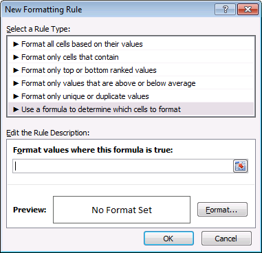
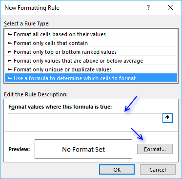
- Press with left mouse button on "Use a formula to determine which cells to format"
- Press with left mouse button on "Format values where this formula is true" window.
- Type
=(B3<=$E$3)*(B3>=$E$2)
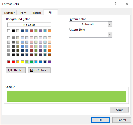
- Press with left mouse button on Format button
- Press with left mouse button on "Fill" tab
- Select a color
- Press with left mouse button on OK!
- Press with left mouse button on OK!
2.2 Explaining CF formula
Step 1 - Check if current cell date is smaller than or equal to end date
B3<=$E$2
becomes
39823<=39833
and returns TRUE
Step 2 - Check if current cell date is larger than or equal to start date
B3>=$E$2
becomes
39823>=39823
and returns TRUE.
Step 3 - Multiply boolean values
Both boolean values must be TRUE in order to highlight the cell.
| Boolean | Boolean | Multiply | Add |
| FALSE | FALSE | 0 (zero) | 0 (zero) |
| FALSE | TRUE | 0 (zero) | 1 |
| TRUE | TRUE | 1 | 2 |
The parentheses make sure that the order of calculation is correct.
(B3<=$E$3)*(B3>=$E$2)
becomes
TRUE*TRUE
and returns 1 which is equivalent to TRUE. Cell B3 is highlighted.
3. Highlight dates arranged in a row

This example demonstrates how to highlight dates arranged horizontally in a row. In fact, the conditional formatting formula is exactly the same. There is no difference between this formula and the formula above.
Conditional formatting formula in cell range B6:F6:
This formula is the same as the above (not the cell references though), the difference is that it is applied to a horizontal cell range.
What is a cell reference?
A cell reference lets you "fetch" and use values in other cells in a formula.
There are two types of cell references:
- A1-style reference
- R1C1 reference
The A1-style reference is the default style in Excel, it names columns by letters from A to Z. After Z it starts over with AA, AB, and so on until XFD. Rows are numbered from 1 to 1048576, older Excel versions use less row numbers.
The R1C1-style uses row number and column number like: R1C1, R2C5 and R10C15. Rows are labeled R1, R2, R3 and so on, columns are labeled C1, C2, C3 etc.
The A1-style reference notation is the most common one, here are some examples:
A1 - single cell reference on the same worksheet
A1:D5 - reference to a cell range on the same worksheet
Budget!Z3 - a single cell reference to worksheet Budget
'Budget 2050'!A3 - a single cell reference to a worksheet containing a space character
What types of A1-style cell references are there?
There are two types of cell references:
- Relative cell references
- Absolute cell references
The examples above contain both relative and absolute relative cell references. The $ dollar character lets you an absolute cell reference meaning you can lock a cell reference horizontally, vertically or both. Here is one example:
A$1 has a relative column reference but an absolute row reference, this means that the column letter may change if the cell is copied and pasted to cells in another column than A. The difference between relative and absolute cell references is important to understand when dealing with conditional formatting formulas.
4. Highlight records

Conditional formatting formula in cell range A7:D16:
This formula is almost the same as the one described in section 1 "Highlight dates based on a a start and end date", see the formula explanation for mor details above in section 1. The cell references are "locked" to column B which is why there is a dollar sign in front of $B7. That makes the entire row highlighted if the date cell is in the date range.
What is a Boolean value?
A Boolean value in Excel is a value that can only be TRUE or FALSE. It represents binary logic and is the result of a logical expression using logical operators or a result of a few Excel functions that I'll discuss below.
Mastering Boolean logic and logical expressions is key to manipulating data and controlling workflow in Excel.
What is binary logic?
Binary logic refers to values having one of two states, TRUE or FALSE. This allows Boolean algebra in Excel using logical operators.
What is a logical expression?
A logical expression is a statement that evaluates to TRUE or FALSE. For example:
=A1<4
These expressions use comparison operators to evaluate a condition and produce a Boolean result.
What are the comparison operators?
= - equal sign
< - less than sign
> - greater than sign
These operators let you build more operators like this:
<> - not equal to
<= - less than or equal to
>= - greater than or equal to
These comparison operators let you create logical expressions like: A2<>5 meaning if the value in cell A2 is not equal to 5, the result is either TRUE or FALSE.
5. Put highlighted values on top

How to sort conditionally formatted cells?
Conditionally formatted cells are great, however, it can be tedious and time consuming to spot highlighted values while scrolling through all data if you work with really large lists.
This trick lets you put highlighted values on top of the list so you can easily find and access them. Here is how you can quickly sort highlighted records to the top of the list:
- Select cell range A6:C15
- Press with right mouse button on on cell range
- Press with left mouse button on "sort"
- Press with left mouse button on "Put selected cell color on top"

All highlighted records are on top.

Get excel *.xls file
highlight-dates-in-range-using-conditional-formatting2.xls
(Excel 97-2003 Workbook *.xls)
6. How to highlight weekends

Conditional formatting formula:
6.1 How to apply conditional formatting to cell range C3:C20
- Select cell range C3:C20.
- Go to tab "Home" on the ribbon.
- Press with left mouse button on the "Conditional Formatting" button.
- Press with left mouse button on "New Rule.." to open a dialog box.
- Press with left mouse button on "Use a formula to determine which cells to format".
- Type the formula. (See above).
- Press with left mouse button on "Format..." button and choose a formatting.
- Press with left mouse button on OK button twice.
6.2 Explaining conditional formatting formula
Step 1 - Identify day of the week
The WEEKDAY function returns 1 to 7 based on a date's day of the week, the second argument tells the function which day a week begins on. Using 2 as the second argument makes the week start on a Monday.
WEEKDAY(C3,2)
becomes
WEEKDAY(43101,2)
and returns 1.
The number calculated by the WEEKDAY function tells us which day of week a date is:
1 - Monday
2 - Tuesday
3 - Wednesday
4 - Thursday
5 - Friday
6 - Saturday
7 - Sunday
Step 2 - Check if the number is larger than 5
The larger than sign checks if the weekday function is larger than 5. If the number is larger than 5 then it must be a Saturday or Sunday, see list above.
WEEKDAY(C3,2)>5
becomes
1>5 and returns FALSE.
Step 3 - Boolean value determines if the cell is highlighted
If the logical expression returns TRUE then the cell is highlighted and FALSE nothing happens.
6.3 How to highlight record when a date falls on a weekend
Conditional formatting formula applied to cell range B3:D20
This formula is almost as the first formula, except there is a dollar sign in front of the B (column number). This makes the column absolute meaning the cell reference doesn't change when the Conditional Formatting moves to the next column. It only changes when it moves to a new row.
Example,
| Cell | Formula |
| B3 | =WEEKDAY($B3,2)>5 |
| C3 | =WEEKDAY($B3,2)>5 |
| D3 | =WEEKDAY($B3,2)>5 |
| B4 | =WEEKDAY($B4,2)>5 |
| C4 | =WEEKDAY($B4,2)>5 |
| D4 | =WEEKDAY($B4,2)>5 |
7. How to highlight dates based on day of week

The TEXT function converts a value to text based on formatting code. The second argument "DDDD" converts the date to day of week.
TEXT(B3,"DDDD")
becomes
TEXT(43101,"DDDD")
and returns Monday.
The equal sign checks if the value is equal to cell $D$3. The dollar signs make sure that cell reference $D$3 doesn't change. Each cell in range B3:B14 is evaluated and if they are equal the logical expression returns a boolean value: TRUE or FALSE.
TEXT(B3,"DDDD")=$D$3
becomes
"Monday"="Monday" and returns TRUE. This highlights cell B3.
7.1 How to apply conditional formatting to a cell range
- Select cell range.
- Go to tab "Home"
- Press with left mouse button on "Conditional Formatting" button.
- Press with left mouse button on "New Rule..."
- Select "Use a formula to determine which cells to format"
- Type the formula in field "Format values where this formula is true:"
- Press with left mouse button on "Format" button, then pick a formatting.
- Press with left mouse button on OK button.
- Press with left mouse button on OK button.
7.2 Highlight records based on day of week

Column B contains all the dates we want to be evaluated, we need to make sure that the conditional formatting formula is locked to column B. A dollar sign in front of column B is what we need.
8. Highlight current date
Cell range B3:B14 has conditional formatting applied, the formula checks if the date is today.
Conditional formatting formula:
A conditional formatting formula must evaluate to TRUE or FALSE or their equivalents any number or 0 (zero).
The TODAY function returns today's date. The equal sign compares the value to the date in cell B3 and returns TRUE or FALSE.
8.1 How to apply conditional formatting to a cell range
- Select cell range.
- Go to tab "Home"
- Press with left mouse button on "Conditional Formatting" button.
- Press with left mouse button on "New Rule..."
- Select "Use a formula to determine which cells to format"
- Type the formula in field "Format values where this formula is true:"
- Press with left mouse button on "Format" button, then pick a formatting.
- Press with left mouse button on OK button.
- Press with left mouse button on OK button.
8.2 Highlight records based on date being today
Conditional formatting formula:
This CF-formula is applied to cell range B3:D12.
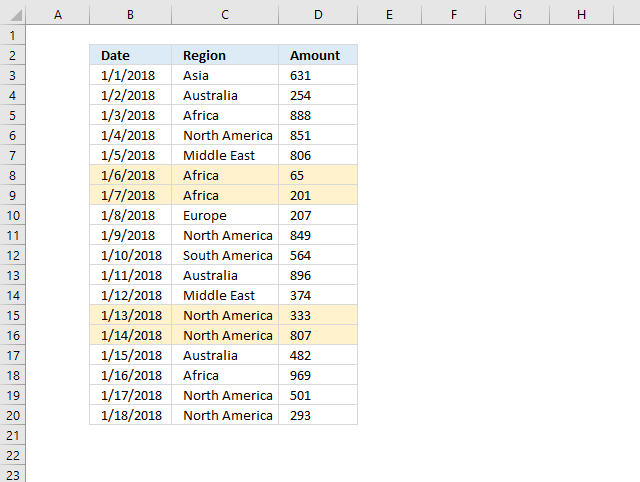
9. How to highlight MAX and MIN value within a month
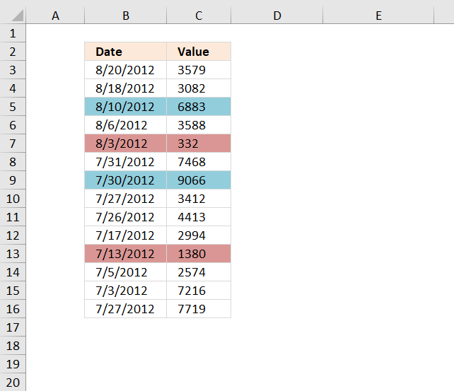
The image above shows rows highlighted based on value in column C being the largest or smallest in that particular month.
Conditional formatting formula (Max)
Conditional formatting formula (Min)
9.1 Explaining CF formula (Max)
Step 1 to 3 make sure that values from the correct year and month are extracted based on the date of the current row.
Step 1 - Compare year to dates
The YEAR function returns the year from an Excel date.
YEAR($B$3:$B$16)= YEAR($B3))
becomes
YEAR({41141; 41139; 41131; 41127; 41124; 41121; 41120; 41117; 41116; 41107; 41103; 41095; 41093; 41117})= YEAR(41141))
and returns
{TRUE; TRUE; TRUE; TRUE; TRUE; TRUE; TRUE; TRUE; TRUE; TRUE; TRUE; TRUE; TRUE; TRUE}.
Step 2 - Compare month to dates
The MONTH function returns a number representing the month from an Excel date.
MONTH($B$3:$B$16)=MONTH($B3)
becomes
MONTH({41141; 41139; 41131; 41127; 41124; 41121; 41120; 41117; 41116; 41107; 41103; 41095; 41093; 41117})=MONTH(41141)
and returns
{TRUE; TRUE; TRUE; TRUE; TRUE; FALSE; FALSE; FALSE; FALSE; FALSE; FALSE; FALSE; FALSE; FALSE}.
Step 3 - Multiply arrays
Both conditions must be met in order to extract the number, we apply AND-logic if we multiply the arrays.
(YEAR($B$3:$B$16)= YEAR($B3))* (MONTH($B$3:$B$16)
becomes
{TRUE; TRUE; TRUE; TRUE; TRUE; TRUE; TRUE; TRUE; TRUE; TRUE; TRUE; TRUE; TRUE; TRUE}*{TRUE; TRUE; TRUE; TRUE; TRUE; FALSE; FALSE; FALSE; FALSE; FALSE; FALSE; FALSE; FALSE; FALSE}
and returns
{1;1;1;1;1;0;0;0;0;0;0;0;0;0}.
Step 4 - Convert boolean values
The IF function returns row number if the logical expression evaluates to TRUE and nothing "" if FALSE.
IF((YEAR($B$3:$B$16)= YEAR($B3))* (MONTH($B$3:$B$16)=MONTH($B3)), $C$3:$C$16, "")
becomes
IF({1;1;1;1;1;0;0;0;0;0;0;0;0;0}, $C$3:$C$16, "")
and returns
{3579; 3082; 6883; 3588; 332; ""; ""; ""; ""; ""; ""; ""; ""; ""}.
Step 5 - Get largest number from array
The MAX function returns the maximum value from a cell range or array.
MAX(IF((YEAR($B$3:$B$16)= YEAR($B3))* (MONTH($B$3:$B$16)=MONTH($B3)), $C$3:$C$16, ""))
becomes
MAX({3579; 3082; 6883; 3588; 332; ""; ""; ""; ""; ""; ""; ""; ""; ""})
and returns 6883.
Step 6 - Compare the largest value to current value
The equal sign compares the values and returns TRUE if they match.
MAX(IF((YEAR($B$3:$B$16)= YEAR($B3))* (MONTH($B$3:$B$16)=MONTH($B3)), $C$3:$C$16, ""))=$C3
becomes
6883=3579
and returns FALSE. Row 3 is not highlighted.
10. Highlight odd/even months
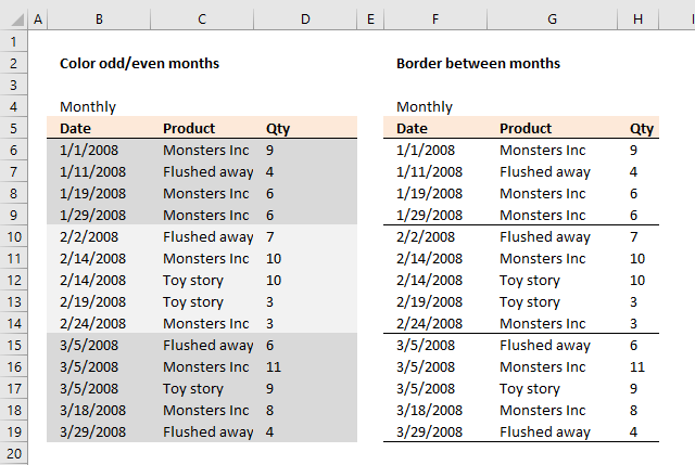
Color odd months
Conditional formatting formula:
10.1 Explaining CF formula in cell B6
Step 1 - Calculate number of month
The MONTH function returns a number representing a month based on a date. 1 = January, 2 = February ... 12 = December.
MONTH($B6)
becomes
MONTH(1/1/2008)
becomes
MONTH(39448)
and returns 1. 1 = January.
Step 2 - Calculate remainder
The MOD function returns the remainder after a number is divided by a divisor.
MOD(MONTH($B6),2)
becomes
MOD(1, 2)
and returns 1.
In cell B10 the date changes to 2/2/2008. MOD(MONTH($B6),2) becomes MOD(2,2) and returns 0 (zero). This cell is not highlighted with this specific color.
10.2 How to apply conditional formatting
- Select cell range B6:D19
- Go to tab "Home" on the ribbon
- Press with mouse on "Conditional Formatting" button
- Press with mouse on "New Rule.."
- Select "Use a formula to determine which cells to format"
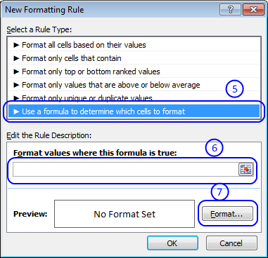
- Type =MOD(MONTH($B6),2) in field "Format values where this formula is true:"
- Then press with left mouse button on "Format..." button
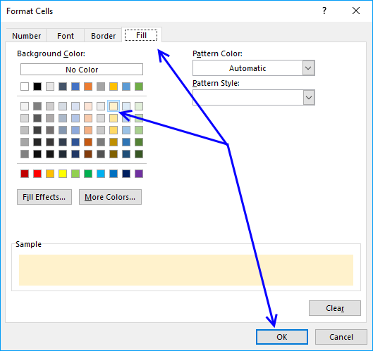
- Go to tab "Fill"
- Pick a color
- Press with left mouse button on OK button
- Press with left mouse button on OK button to return to Excel.
10.3 Color even months
Conditional formatting formula:
The NOT function returns the boolean opposite to the given argument. The numerical equivalent to boolean value TRUE is 1 and FALSE is 0 (zero).

10.4 Highlight odd years
Conditional formatting formula:
The YEAR function returns the year based on a date.
10.5 Highlight even years
Conditional formatting formula:

10.6 Line between months - conditional formatting
Conditional formatting formula:

10.7 Line between years - conditional formatting
Conditional formatting formula:
11. Highlight overlapping date ranges using conditional formatting
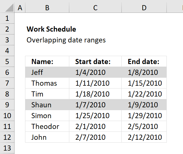
The image above demonstrates a conditional formatting formula that colors a record if there is at least one record that overlaps.
The first and fourth record are highlighted because the date ranges overlap. 1/4/2010 - 1/8/2010 overlaps with 1/7/2010 - 1/9/2010.
Here are the steps needed to create a conditional formatting formula
- Select cell range B6:D12.
- Press with left mouse button on "Home" tab.
- Press with left mouse button on "Conditional Formatting" button.
- Press with left mouse button on "New Rule..".
- Press with left mouse button on "Use a formula to determine which cells to format".
- Type =SUMPRODUCT(($C6<=$D$6:$D$12)*($D6>=$C$6:$C$12))>1 in "Format values where this formula is TRUE" window.
- Press with left mouse button on "Format.." button.
- Press with left mouse button on "Fill" tab.
- Pick a color. This color is used to highlight records that overlap.
- Press with left mouse button on "OK".
- Press with left mouse button on "OK".
- Press with left mouse button on "OK".
Explaining conditional formatting formula
=SUMPRODUCT(($C6<=$D$6:$D$12)*($D6>=$C$6:$C$12))>1
Step 1 - Filter records where ($C6<=$D$6:$D$12) is TRUE
$C6<=$D$6:$D$12 returns an array of TRUE and/or FALSE if date in cell C6 is smaller or equal to each date in $D$6:$D$12.
All dates in$D$6:$D$12 are larger than $C6 so the returning array is (TRUE, TRUE, TRUE,TRUE, TRUE, TRUE,TRUE)
Step 2 - Filter records where ($D6>=$C$6:$C$12) is TRUE
($D6>=$C$6:$C$12) returns an array of TRUE and/or FALSE if date in cell D6 is bigger or equal to each date in $C$6:$C$12.
The returning array is (TRUE, FALSE, FALSE,TRUE, FALSE, FALSE,FALSE)
Step 3 - Putting it all together
($C6<=$D$6:$D$12)* ($D6>=$C$6:$C$12)) returns the following array (1,0,0,1,0,0,0).
That means array number one and four is overlapping C6:D6) but in this case we just want to know if any date range is overlapping.
=SUMPRODUCT(($C6<=$D$6:$D$12)*($D6>=$C$6:$C$12)) sums the array (1,0,0,1,0,0,0) and returns 2.
If the formula returns a number bigger than one there is at least one overlapping date range.
=SUMPRODUCT(($C6<=$D$6:$D$12)*($D6>=$C$6:$C$12))>1 returns TRUE or FALSE.
Recommended articles
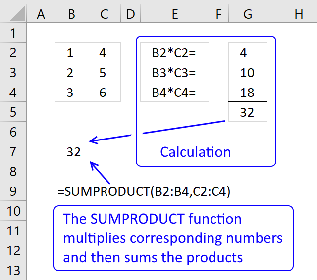
The SUMPRODUCT function calculates the product of corresponding values and then returns the sum of each multiplication.
Get excel *.xls file
highlight overlapping dates.xls
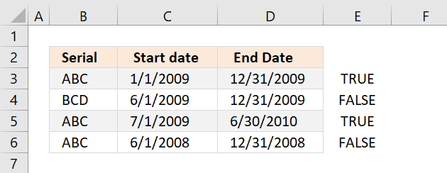
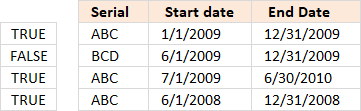
12. Highlight records based on overlapping date ranges and a condition
Hi, I have a situation where I want to count if this value is duplicate and if it the dates are overlapping as well. Is there anyway to work this out?
eg
Serial | Start date | End Date
ABC | 01.01.2009 | 31.12.2009
BCD | 01.06.2009 | 31.12.2009
ABC | 01.07.2009 | 30.06.2010
So it should list the first and third entry.
Answer:
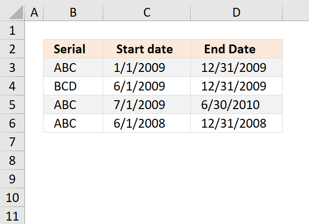
The image above demonstrates a conditional formatting formula that highlights records based on a condition (column B) and date ranges (column C and D).
Records on row 3 and 5 are highlighted, they share the same condition in column B and their date ranges overlap.
How to apply conditional formatting formula to the data set
- Select a cell range
- Press with left mouse button on the "Home" tab
- Press with left mouse button on "Conditional Formatting" button
- Press with left mouse button on "New Rule.."
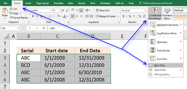
- Press with left mouse button on "Use a formula to determine which cells to format"
- Type =SUMPRODUCT(($C3<=$D$3:$D$6)*($D3>=$C$3:$C$6)*($B3=$B$3:$B$6))>1 in "Format values where this formula is TRUE" window.
- Press with left mouse button on "Format.." button
- Press with left mouse button on "Fill" tab
- Select a color for highlighting cells.
- Press with left mouse button on "Ok"
- Press with left mouse button on "Ok"
- Press with left mouse button on "Ok"
Explaining CF formula in cell B3
The formula is a conditional formatting formula, however, you can enter it in cell E3. Then copy the cell and paste to cells below.
Select cell E3 and then start the "Evaluate Formula" tool on the "Formula" tab on the ribbon.
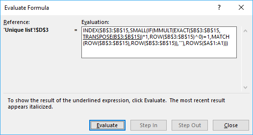
Press with left mouse button on "Evaluate" button to go through each calculation step.
Step 1 - Check if cells are equal to cell value
The equal sign lets you compare a cell value with a range. If it is the same the logical expression returns TRUE, if not FALSE.
 $B3 is locked to column B, however, the row number changes as the CF formula is applied to cells below.
$B3=$B$3:$B$6
becomes
"ABC "={"ABC ";"BCD ";"ABC ";"ABC "}
and returns {TRUE;FALSE;TRUE;TRUE}.
Step 2 - Check if date ranges overlap
The following two logical expressions check which date ranges overlap with the first record. The parenthes make sure that the order of calculation is correct. We want the comparisons to be performed first and then multiply the arrays.
($C3<=$D$3:$D$6)*($D3>=$C$3:$C$6)
becomes
(39814<={40178;40178;40359;39813})* (40178>={39814;39965;39995;39600})
 becomes
{TRUE;TRUE;TRUE;FALSE}* {TRUE;TRUE;TRUE;TRUE}
and returns {1;1;1;0}
Step 3 - Multiply arrays
($C3<=$D$3:$D$6)*($D3>=$C$3:$C$6)*($B3=$B$3:$B$6)
 becomes
{TRUE;FALSE;TRUE;TRUE}* {1;1;1;0}
and returns {1;0;1;0}
Step 4 - Sum values in array
SUMPRODUCT(($C3<=$D$3:$D$6)*($D3>=$C$3:$C$6)*($B3=$B$3:$B$6))
becomes
SUMPRODUCT({1;0;1;0})
and returns 2.
Step 5 - Check if sum is larger than 1
SUMPRODUCT(($C3<=$D$3:$D$6)*($D3>=$C$3:$C$6)*($B3=$B$3:$B$6))>1
becomes
2>1
and returns TRUE. Cell B3 is highlighted.
Get Excel *.xlsx file
duplicate values and overlapping dates.xlsx
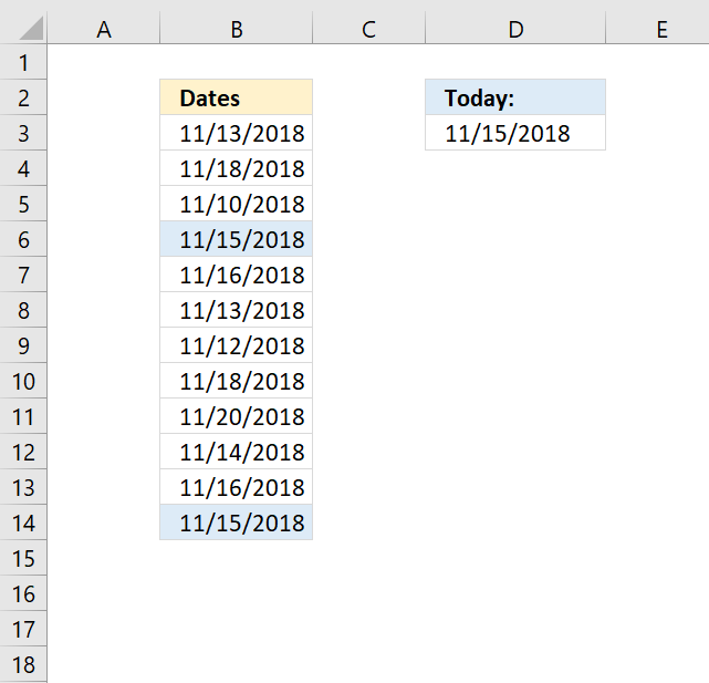
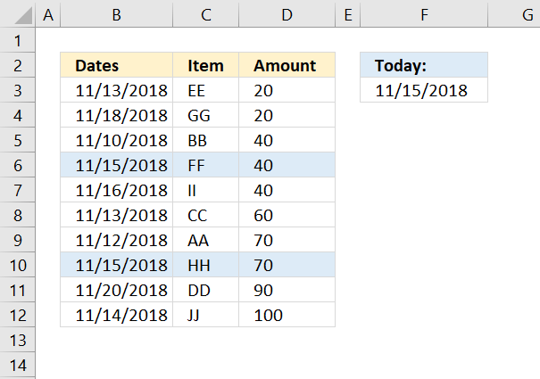
13. Highlight date ranges overlapping selected record - VBA
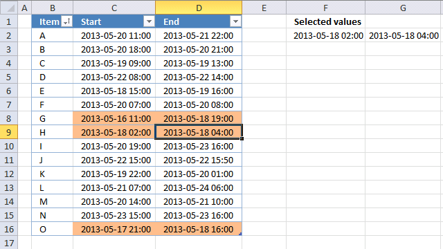
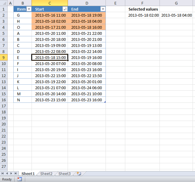
This article demonstrates event code combined with Conditional Formatting that highlights overlapping date ranges based on the selected date range.
This method will automatically highlight the selected date range and all other overlapping date ranges, press with left mouse button on any another date range to highlight it and it's overlapping date ranges as well.
Event code is basically a VBA macro that is run when an event is triggered, it can be a specific worksheet being activated or a cell being selected among many other things.
The image above shows cell D9 selected, the event code then copies the date range in cell range C9:D9 to cell range F2:G2. A conditional formatting formula uses the values in cells F2 and G2 to highlight other date ranges in the Excel Table that overlaps.
Table of Contents
-
- Create an Excel Table
- Event code
- Where to put the event code?
- Conditional formatting formula
- Explaining CF formula
- Sort highlighted values
- Hide values in cell F2:G2
13.1. Create an Excel Table

An Excel Table has many great features, the one we are most interested in for today's tutorial is "structured references". It is basically a cell reference to an Excel Table, however, more advanced but still easy to construct.
This makes it possible to apply conditional formatting to all data in Excel Table even if data is added or deleted.
- Select any cell in your data set.
- Press short cut keys CTRL + T and "Create Table" dialog box appears, see image above.
- Enable checkbox if your table contains header names.
- Press with left mouse button on OK to apply settings and create Excel Table.
The cell formatting changes to indicate that the data set is now an Excel Table, you have the option to change the Table style if you want.
Go to tab "Table Design" on the ribbon, press with left mouse button on the button shown in the image below to expand the list of Table Styles.

Hover over a table style and your Excel Tables instantly changes to show what it looks like. This makes it easy to preview a table style and pick one that you like in no time.
13.2. Event code
The code below must be placed in a worksheet module to work properly, you cant put it in a regular module. This macro is triggered when the user selects any cell in columns C or D.
It copies the selected dates to cell range F2:G2 in order to highlight the appropriate dates using conditional formatting in the next step.
'Event code
Private Sub Worksheet_SelectionChange(ByVal Target As Range)

    'Check if selected cell is in column C or D
    If Not Intersect(Target, Range("C:D")) Is Nothing Then

        'Save dates from column C and D to cell range F2:G2
        Range("F2:G2") = Range("C" & Target.Row & ":D" & Target.Row).Value
    End If
End Sub
13.3. Where to put the event code?

The image above shows the Visual Basic Editor, it contains the project explorer to the left and a window to the right showing the VBA code if any.
- Copy the above event code. (CTRL + c).
- Press with right mouse button on on sheet name.
- Press with left mouse button on "View code" and Visual Basic Editor appears with the corresponding worksheet module open.
- Paste event code, see image above. (CTRL + v).
- Exit VB Editor and return to Excel.
13.4. Conditional formatting formula

- Select date ranges in the Excel Table, the image above shows cell range C2:D16 selected.
- Go to tab "Home" on the ribbon.
- Press with left mouse button on the "Conditional formatting" button located on the ribbon.
- Press with left mouse button on "New Rule..".
- Select Rule Type: "Use a formula to determine which cells to format". See image above.
- Enter the Conditional Formatting formula shown below these steps.
- Press with left mouse button on the"Format..." button.
- Press with left mouse button on tab "Fill".
- Pick a fill color.
- Press with left mouse button on Ok.
- Press with left mouse button on OK
Conditional formatting formula
13.4.1 Explaining CF formula

I recommend that you enter the formula in cell H2 to easily see how the CF formula works. Copy cell H2 and paste to cell range H3:H16.
Excel has a built-in tool named "Evaluate Formula" that allows you to see formula calculations for the selected cell step by step.

Go to tab "Formulas" on the ribbon. Press with mouse on the "Evaluate Formula" button. A dialog box appears, see image above.
The "Evaluate" button takes you through the formula calculations step by step, the underlined part of the formula is what will be evaluated next time you press the Evaluate" button.
Italic text shows the result. Press with left mouse button on the "Evaluate" button repeatedly until you are pleased or the formula has been completely calculated. Press with left mouse button on "Close" button to dismiss the dialog box.
I have described each step in the formula calculation entered in cell H2 below. The formula corresponds to the CF formula applied to cell range C2:D2.
Step 1 - Check if date is smaller than selected date in cell F2
The less than sign checks if the date in cell F2 is smaller than the date in cell D2. The result is the boolean values True or False.
Excel handles dates as numbers, however, cell formatting shows them as dates. For example, enter 1 in any cell. Select the cell and press CTRL + 1 to open the "Format cells" dialog box.
Apply any date formatting, press with left mouse button on OK button. The cell now shows 1/1/1900, this proves to you that Excel handles dates as numbers. A date less than another date means it is a smaller number meaning it is earlier than the other date.
Time is the decimal part of a number. 1/24 is an hour.
Cell reference $F$2 is an absolute cell reference meaning it does not change when the cell is copied to cells below, this applies also to Conditional formatting formulas as well.
Cell reference $D2 is only locked to the column and the row number is relative meaning it changes from cell to cell.
$F$2<$D2
becomes
41414.4583333333<41415.9166666667
and returns boolean value True.
Step 2 - Check if date is larger than selected date in cell G2
$G$2>$C2
becomes
41415.9166666667>41414.4583333333
and returns TRUE.
Step 3 - Multiply results
Multiplying boolean values is the same as applying AND-logic. True * True = 1, True * False = 0 and False * False = 0.
The numerical equivalent to True is 1 and False is 0 (zero).
The parentheses allow you to control the calculation, we want to evaluate the less than and larger than signs before we multiply the results.
($F$2<$D2)*($G$2>$C2)
becomes
TRUE * TRUE
and returns TRUE. Cell C2 and cell D2 will be highlighted by the Conditonal Formatting tool.
13.5. Sort highlighted values
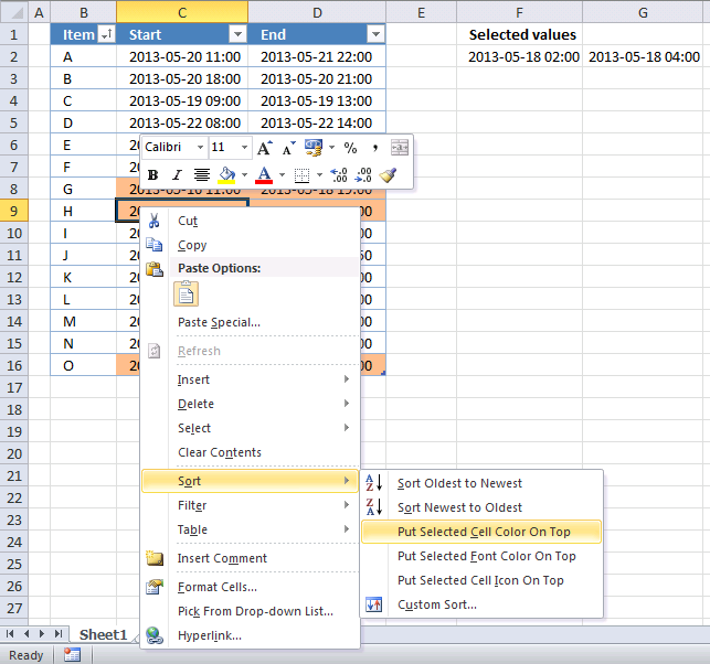
Finding conditionally formatted values in a large Excel Table is not easy but there is a way that can be useful. This method sorts all conditionally formatted values at the top of the Excel Table.
- Press with right mouse button on on a cell that is highlighted.
- Press with mouse on Sort, see image above.
- Press with mouse on "Put selected cell color on top".
13.6. Hide values in cell F2:G2
You can hide the dates if you don't want the selected dates to be shown in cell range F2:G2. The following steps demonstrate how to format cells manually.
- Select cell F2:G2
- Press with right mouse button on on cells.
- Press with left mouse button on "Format cells..."
- Select category: "Custom"
- Type ;;;
- Press with left mouse button on OK
They will hide values in cell range F2:G2, however, they still exist there. You can check that by selecting either cell F2 or G2 and the values show up in the formula bar.

The formula bar shows a number with decimals, this is how Excel handles dates. They are simply numbers formatted as dates, 0 (zero) is 1/1/1900 and 1/1/2000 is 36526.
Time values are decimal numbers. 12:00 A.M. is 0 (zero) and 1/24 is 01:00 A.M. 23/24 is 11:00 P.M.
Combine both date numbers and time numbers and you get 36526.5 equals 1/1/2000 12:00 P.M.
Recommended reading
Built-in conditional formatting
Data Bars Color scales IconsHighlight cells rule
Highlight cells containing stringHighlight a date occuring
Conditional Formatting Basics
Highlight unique/duplicates
Top bottom rules
Highlight top 10 valuesHighlight top 10 % values
Highlight above average values
Basic CF formulas
Working with Conditional Formatting formulasFind numbers in close proximity to a given number
Highlight empty cells
Highlight text values
Search using CF
Highlight records – multiple criteria [OR logic]Highlight records [AND logic]
Highlight records containing text strings (AND Logic)
Highlight lookup values
Unique distinct
How to highlight unique distinct valuesHighlight unique values and unique distinct values in a cell range
Highlight unique values in a filtered Excel table
Highlight unique distinct records
Duplicates
How to highlight duplicate valuesHighlight duplicates in two columns
Highlight duplicate values in a cell range
Highlight smallest duplicate number
Highlight more than once taken course in any given day
Highlight duplicates with same date, week or month
Highlight duplicate records
Highlight duplicate columns
Highlight duplicates in a filtered Excel Table
Compare
Highlight missing values between to columnsCompare two columns and highlight values in common
Compare two lists of data: Highlight common records
Compare tables: Highlight records not in both tables
How to highlight differences and common values in lists
Compare two columns and highlight differences
Min max
Highlight smallest duplicate numberHow to highlight MAX and MIN value based on month
Highlight closest number
Dates
Advanced Date Highlighting Techniques in ExcelHow to highlight MAX and MIN value based on month
Highlight odd/even months
Highlight overlapping date ranges using conditional formatting
Highlight records based on overlapping date ranges and a condition
Highlight date ranges overlapping selected record [VBA]
How to highlight weekends [Conditional Formatting]
How to highlight dates based on day of week
Highlight current date
Misc
Highlight every other rowDynamic formatting
Advanced Techniques for Conditional Formatting
Highlight cells based on ranges
Highlight opposite numbers
Highlight cells based on coordinates
Excel categories
85 Responses to “Advanced Date Highlighting Techniques in Excel”
Leave a Reply
How to comment
How to add a formula to your comment
<code>Insert your formula here.</code>
Convert less than and larger than signs
Use html character entities instead of less than and larger than signs.
< becomes < and > becomes >
How to add VBA code to your comment
[vb 1="vbnet" language=","]
Put your VBA code here.
[/vb]
How to add a picture to your comment:
Upload picture to postimage.org or imgur
Paste image link to your comment.
Hi, I have a situation where I want to count if this value is duplicate and if it the dates are overlapping as well. Is there anyway to work this out?
eg
Serial | Start date | End Date
ABC | 01.01.2009 | 31.12.2009
BCD | 01.06.2009 | 31.12.2009
ABC | 01.07.2009 | 30.06.2010
So it should list the first and third entry.
[...] Highlight duplicate values and overlapping dates in excel Filed in Excel on Oct.09, 2010. Email This article to a Friend adam asks: [...]
Adam,
read this post: Highlight duplicate values and overlapping dates in excel
Thanks. It works perfectly.
I want to do something similar but only if the value in column B is the same as the previous or subseqhent row. In other words, column B might be something like an employee number (5 in this case) and I only want to look for overlapping dates across the same employee number like this.
# Start date End date
5 2/11/1995 10/22/2002
5 10/22/2002 12/31/9999
The above overlap as does the below
5 2/11/1995 10/22/2002
5 10/19/2002 12/31/9999
Can I do this in excel with the condition that the employee number Key (5 in this case) has to match?
PJ,
Conditional formatting formula:
=SUMPRODUCT(($C6<=$D$6:$D$12)*($D6>=$C$6:$C$12)*($B6=$B$6:$B$12))>1
Get the Excel file
Hi Oscar,
Please help me.
In due date i used this formula to track if the employee already exceed in her Inactive status.
NOTE: g1=DATE TODAY
=IF(E2=$G$2+5,"5 DAYS BEFORE DUE",IF(E2=$G$2,"EXPIRED",IF(E2<$G$1,"EXCEEDED", "--"))
If ever the employee Back to work from Inactive status. I would like to erase automatic the "EXCEEDED" in column Due date.
What formula can i used? Please help me
HRID LName Status Start End Due Date
57456 RODRIGUEZ INACTIVE 6-Jan-12 15-Jan-12
65153 MENDOZA INACTIVE 1-Sep-08 9-Apr-12
57456 RODRIGUEZ BACK TO WORK 15-Jan-12 5-Jan-12
57613 JOSE INACTIVE 16-Mar-10 8-Jun-11
Ana,
Get the Excel *.xlsx file
Ana.xlsx
Oscar,
Thank you so much for your help... This is great...
Thank you Mr.Genius
Hi Oscar,
If possible, if ever I can add Separated status in column C(Status). If ever she BACK TO WORK or SEPARATED the "EXCEEDED" in column Due date automatic erase.Please advise
Thank you
Oscar,
Please help me....What formula can i used?
Oscar,
Please help.....
Ana,
I don´t think I understand. Your first question:
If ever the employee Back to work from Inactive status. I would like to erase automatic the "EXCEEDED" in column Due date.
Your next question:
add Separated status in column C(Status). If ever she BACK TO WORK or SEPARATED the "EXCEEDED" in column Due date automatic erase.
Anyway I tried, get the Excel *.xlsx file:
https://www.get-digital-help.com/wp-content/uploads/2010/10/ANA1.xlsx
Oscar,
This is awesome formula Oscar. Thank you so much .
THANK YOU........
ah great formula Oscar! interesting...
Oscar,
I have i problem in how to compute the total interval of date and time .And i would like the output like this: 1(for day) 02:00(for hours). Please help......
Example.
A-start B. End C.Output
1/23/2012 01:00pm 1/24/2012 03:00pm 1 2:00
mei,
Formula in C2:
Oscar,
I try the formula but something error appear.
"The formula you typed contain an error"
Please oscar help me.......
Confused :( Both formulas looks like same. do i have to replace MAX part in second formula with MIN ?? . Also guide me how to use them, where should i insert the formula?
Thank you very much Oscar
srini
srinivas,
Confused Both formulas looks like same. do i have to replace MAX part in second formula with MIN ??
Yes, you are right! It is now corrected.
Also guide me how to use them, where should i insert the formula?
It is a conditional formatting formula.
How to apply the conditional formatting formula in excel 2007:
1. Select cell range B2:B159
2. Go to tab "Home"
3. Press with left mouse button on the "Conditional formatting" button
4. Press with left mouse button on "New rule..."
5. Press with left mouse button on "Use formula to determine which cells to format"
6. Type formula
7. Press with left mouse button on "Format..." button
8. Select a color.
9. Press with left mouse button on OK twice.
Repeat steps and use the second formula and preferbly another color.
Thank you very much Oscar. It is now clear :)
Hi Oscar,
I try the formula but something error appear.
"The formula you typed contain an error" this is the error appeared in my sheet.
Please help
mei,
You may have to adjust the "HH:MM" part depending on your regional settings. HH is hours and MM is minutes.
Oscar,
Thank you so much.....
Hi Oscar,
I have difficulty finding out the overlapping of dates. see example:
EMP ID TYPE OF LEAVE START END
1234 Sick 13-Mar-2012 13-Mar-2012
1234 Sick 10-Mar-2012 18-Mar-2012
5678 Annual 11-Feb-2012 12-Feb-2012
5678 Annual 12-Feb-2012 15-Feb-2012
5678 Annual 09-Feb-2012 18-Feb-2012
I'm checking for over 4,000 records. PLEASE HELP!
THANK YOU SO MUCH.
Lucy,
Is this what you are looking for?
Lucy.xlsx
Yes is there any formula to highlight the overlapping dates?
Thanks!
Lucy,
the formula I provided highlights overlapping dates only if the EMP ID is the same.
This formula highlights records with overlapping dates.
SUMPRODUCT(($C2<=$D$2:$D$6)*($D2>=$C$2:$C$6))>1
Hey Oscar,
I am trying to do something similar but cannot figure it out. if you could help I would really appreciate it as I need to fix our database this week & remove duplicate
Column J = Ad Id #
Column f = Date
I am trying to highlight all of the cells where the AD ID# was entered for the same date. The AD ID #'s are all unique so my logic is that there should never be the same AD ID entered into the spreadsheet with the same date.
I have tried this formula, but no luck - =SUMPRODUCT(($J2=$J$2:$J$9263))>1
Thanks for your help!Let me
* This formula
=SUMPRODUCT(($J2=$J$2:$J$9263))>1
Hmm I am not sure why the whole formula is not showing up..
I will break it up
=SUMPRODUCT(($J2=$J$2:$J$9263))>1
Carter Mahoney,
Conditional formatting formula:
=SUMPRODUCT(($A2=$A$2:$A$7)*($B2=$B$2:$B$7))>1
Carter-Mahoney.xlsx
hey this formula works perfectly for each month but how do I make it do it by year and month? I have about 2600 lines I have to highlight each max and min value for each month of each year.
Pradeep,
Conditional formatting formula min value:
Conditional formatting formula max value:
Get the Excel *.xlsx file
Highlight-max-and-min-value-in-every-month.xlsx
I'd like to do this for a row instead of a column, but I'm stuck. (I replace 'A1' with '1:01'.) Can this be done?
Kate,
I have have added more content, I hope it will answer your question.
Hello Oscar,
thank you so much for your formula, it has helped me a lot so far.
i work for a small car rental company, and im having another problem with applying your code.
i will try to explain it as clearly as possible without having to share the complete file.
I have a table that collapses column's.
e.g.
Vehicle License plate - Chauffeur - Date out - Date in - Destination.
these headers are grouped so its easier to look up a vehicle.
these columns repeat 25x.
so far so good,
i have for each vehicle 4 inputs, so it will look like this:
------------(A)--|-(B)-|(C)|(D)|
(1)-------LICENSE|CHAUF|OUT| IN|
(2)INPUT 1
(3)INPUT 2
(4)INPUT 3
(5)INPUT 4
it now correctly marks when a date overlaps for the same vehicle,
(" =SOMPRODUCT(($G3=$G$3:$G$6))>1 "), as it only needs to look up in a small cluster.
but now i have the following issue, we have loads of personal chauffeurs.. (a file of 35 chauffeurs over 25 vehicles)
which need to be checked up in different (divided) colums.
i have prevented planning the same vehicle twice in the same timeframe.
but now i need it to lookup if the chauffeur is not planned twice! (not vehicle dependend!)
EG.
License is column A,E and I
Chauffeur is column B, F and J
Date out is column C, G and K
Date in is column D, H and L
My instinct is telling me this:
=SUMPRODUCT(($C2=$C$2:$C$5+$G$2:$G$5+$K$2:$K$5)*($B2=$B$2:$B$5+$F$2:$F$5+$J$2:$J$5))>1
could you please correct my code?
Robin,
Example with eight columns:
Conditional formatting formula in cell range A6:D12:
Conditional formatting formula in cell range G6:J12:
See attached file:
highlight-overlapping-dates-robin.xls
It would have been a lot easier if you had all records in 4 columns.
Example:
Thank you very Oscar, this formula is working ,
I am using it in range of few hundred and its giving the perfect result. I did adjust a bit to suit for my requirement
=SUMPRODUCT(($C6$C$6:$C$120)*($B6=$B$6:$B$120))>1
I have used the formula as below
=SUMPRODUCT(($C6$C$6:$C$120)*($B6=$B$6:$B$120))>1
Jahid,
I am happy you like it.
PLEASE HOW TO CALCULATE OVERLAPING DAY IN NUMBER
FOR EX.
2/1/2012 5/1/2012
3/1/2012 4/1/2012 2 DAYS OVERLAPING
SAMAN,
read this post: Count overlapping days in a date range
i am trying to do a conditional formatting for a calendar row. (essentially, a gant chart)
i have a schedule table with event in 1st column, start date in 2nd column, end date in 3rd column, and a 2-criteria condition for the event in the 4th column.
how do i condition format the cell row beneath the calendar row so that they are within the start/end date and will be color coded brown or blue based on the 2-criteria? I already have a conditional formatting done for weekends and holidays for the calendar row itself, so hence the new row beneath.
bryan,
Can you provide example data and desired outcome?
Oscar,
Thank you for the reply. Further info provided:
I have a schedule table with 4 columns.
1. Column D has the event name
2. Column E has the Start date
3. Column F has the End date
4. Column G has a drop-down choice of "home" or "out of area"
I have a calendar going from I1:IV1. I have it setup for highlighting federal holidays and weekends for conditional formatting.
I have a row setup beneath the calendar from I3:IV3 that I'd like to conditionally format to reflect based on the start-end date ranges in the schedule table with color coding for "home" or "out of area".
Thank you.
bryan,
Read this: Highlight events overlapping federal holidays
[...] Bryan asks: [...]
Hi
Regarding your section on 'HIGHLIGHT RECORDS', how do I Conditional Format to highlight dates in range that are recognised, but then automatically highlight all cells in the row?
IE: Using your HIGHLIGHT RECORDS example:
Conditional Format (as per your formulae provided) to recognises dates between 10-01-2009 & 20-01-2009
Then automatically highlight COUNTRY & COMPANY once dates recognised by Conditional Formatting.
John-Paul
I don´t understand.
The "Highlight records" example highlights all cells (also country and company) in a row?
Can you explain in greater detail?
Hi,
I am making a Schedule of Project in Excel, Where i am taking 2 column as Start date and End date. While I need that whenever i enters the start date and end date , according to that rows color changes simultaneously..... While after End date column, Next all columns belongs to week wise column. so every cell color changes accordingly with respect to weekwise.
Please let me know how to set a format like this....
Thru which color changes automatically, whenever i enters dates.
Avin
Avin,
I am not following, can you please take a screenshot of your sheet and the desired outcome. Upload to postimage.org. Then add the picture link to your comment.
Hi Oscar,
Great website! Keep up the good work.
I have a question as to how to expand this to the next step. Per your initial example we can see that Jeff in Row 1 and Shaun in Row 4 overlap their work schedule. I would like to know if there were a way, say for instance in Range E6:E12, to display Jeff’s Row number next to Shaun’s name and visa – versa. I can see how this will easily display what record numbers overlap when there is only one overlap in the range. Can we differentiate the records when there are two overlaps? Let’s say Theodor in Row 6 also has an overlap with Thomas in Row 2.
Now the data becomes confusing because we have to determine, from the 4 grayed rows, who overlaps with whom.
Can a formula return the Row value of the “matching” overlap record?
In Jeff’s E6 cell it would indicate “Row 4” as to the matching record, and the reverse for Shaun. Shaun’s E9 cell would indicate “Row 1” as the matching record.
And at the same time Theodor’s E11 cell would reflect “Row 2” for Thomas’s record and Thomas’ E7 cell would show “Row 6” for Theodor.
I haven’t even touched on the tougher one, such as what happens when John in Row 7 has an end date of 2010-01-07, thus overlapping with both Jeff and Shaun!
One step at a time. :)
Thanks
cwrbelis,
Great question!
Read this article:
Identify overlapping records
Hi Oscar, I have what I think is a simple scenario which I thought I could solve using your overlapping date range example but I am not getting the results I expect.
At its simplest form, the cells are:
A1 04/01/2004 B1 08/01/2008
A2 11/01/2003 B2 15/01/2012
in D1 I have {=$B1>=$A2:$B2}
I want a TRUE/FALSE result should the B1 date fall between the date range for A2 (start date) to B2 (end date)
Martin,
Formula in D1:
=(B1>=A2)*(B1<=B2)
Thank you Oscar! Can you elaborate on taking the same dates as whole ranges to compare? So if I wanted a TRUE/FALSE for when the date period starting from A1 and ending at B1 overlaps the start date in A2 and the end date in B2?
Martin,
Can you elaborate on taking the same dates as whole ranges to compare?
That is what the formula in this post does. It compare cell C6 with cell range D6:D12 and cell D6 with cell range C6:C12.
=SUMPRODUCT(($C6<=$D$6:$D$12)*($D6>=$C$6:$C$12))>1
$C6<=$D$6:$D$12 returns an array and $D6>=$C$6:$C$12 returns an array. By multiplying both arrays you check if both values on each row is TRUE. If more than 1 value returns true the whole function returns true. That means there is at least one overlapping date range.
Thanks again Oscar. I apologise for not being clear, in my scenario I am attempting to find out dates that overlap in these cell ranges and to indicate the overlap. I have tried using conditional formatting and formula =SUMPRODUCT(($G9=$G$9:$G$29))>1 but I am still not having much success at all.
In the sample below, below each date are hidden calculations / formula that I want to exclude from the overlapping check, I only wish the cells below to have the overlapping date check applied. I want to know if any DATE START and DATE END overlap, ideally through conditional formatting to highlight the overlapping date ranges.
CELL START CELL DATE END
G9 01/01/2001 P9 01/01/2002
G14 01/02/2001 P14 01/04/2002
G19 01/03/2003 P19 01/04/2004
G24 01/04/2004 P24 01/06/2005
G29 01/09/2005 P29 01/01/2010
Am I failing at this because of the data held underneath each date range, as specifying G9:G29 for example will include cells that I want to exclude. I've tried =SUMPRODUCT(($G9=$G$9+$G$14+$G$19+$G$24+$G$29)>1 but with no success either. Perhaps I should be looking at another formula rather than SUMPRODUCT?
For some reason my previous post was incomplete. The formula's should read:
=SUMPRODUCT(($G9=$G$9:$G$29))>1
and
=SUMPRODUCT(($G9=$G$9+$G$14+$G$19+$G$24+$G$29)>1
Martin,
I hope this helps:
Get the Excel file
overlapping-date-ranges.xlsx
I've tried the above method but only two of my dates actually got highlighted. Is there and issue in Excel 2010?
I have dates in two particular cells and I need a row of dates to highlight a particular color if the dates fall on or between the particular dates. I think the formula for rows above should work but it is not.
Jen
Jen,
I've tried the above method but only two of my dates actually got highlighted. Is there and issue in Excel 2010?
No, it works in excel 2010.
Is there an issue on the attached file? The attached file works here (excel 2010).
Can you provide your Conditional Formatting formula?
Did you check the absolute and relative cell refs in your CF formula?
Here is a pdf of what I'm talking aobut. I've applied the conditional formatting, but the cells that are white (Y7 to AM7) *should* be green.
https://s26.postimg.org/p77hmqeuh/Page_1_Conditional_Formatting_Sample.jpg
Jen,
your CF formula should be:
=(Y7>=$I$7)*(Y7<=$J$7) not =(Y7<=$I$7)*(Y7>=$J$7)
Hi Oscar,
I hope this site is still active.
I'm looking for a formula that will identify/highlight duplicate names within every six week time period.
So if 'John Smith' appears twice within any six week period it would highlight his name.
I only have 2 columns, date and name.
Thanks!
Hi,
I used the above formula and it worked. However when I have some rows having blank dates, it applies the formatting also.
Hi Oscar
I manage our family's shared holiday cottage, and need something almost like your example, but with one difference:
People can arrive on the same day the previous people are departing, so that doesn't count as an overlap.
How do I change the formula?
Thanks a lot!
Anton,
interesting question.
Try this:
It works perfectly!
Thanks a LOT Oscar, your prompt reply is appreciated!
Hi,
In the example with eight columns which is what I am trying to do, is it possible not to have it look at it's own columns but just across?
So the range C&D would only look at the range I&J and report any overlapping ranges between those only?
TIA
Erik
Erik
Conditional formatting formula, cell range A6:D12:
=SUMPRODUCT(($C6<=$J$6:$J$12)*($D6>=$I$6:$I$12)*($B6=$H$6:$H$12))>0
Conditional formatting formula, cell range G6:J12:
=SUMPRODUCT(($I6<=$D$6:$D$12)*($J6>=$C$6:$C$12)*($H6=$B$6:$B$12))>0
There are overlapping date ranges in the first cell range but not highlighted, row 8 and 12.
The same thing with the second cell range, row 8 and 12.
Only row 8 in the first range is highlighted because it overlaps row 12 in the second range.
It works well. Exactly what i needed.Thank you so much =D
Dear Oscar,
How can I do this for the repeating textual items in column A instead of dates? For example, I would like to determine min values for pears, apples, oranges, whereas the series looks like this:
Pear 5.5
Pear 1.2
Apple 3.2
Apple 5.5
Pear 1.2
Orange 6
Apple 3.2
Orange 5.5
Pear 1.2
Thank you in advance.
Best regards,
Goranka
Goranka
Great question.
Array formula in cell E1:
=MIN(IF(D1=$A$1:$A$9,$B$1:$B$9,""))
Array formula in cell E2:
=MIN(IF(D2=$A$1:$A$9,$B$1:$B$9,""))
Array formula in cell E3:
=MIN(IF(D3=$A$1:$A$9,$B$1:$B$9,""))
Hello Oscar, thanks a lot for this helpful website!
I am trying to apply the formula to a wider range than in your illustration. So instead of range "A6:D12", I am trying to apply it to the range "A6:D500" for example, where "A13:D500" are blank rows.
What happens is that all the blank rows get highlighted. Could you please help me with that problem?
Much appreciated
Hi,
would love to know whether there is a formula to find how many days, two dates range, are falling in a certain period.
e.g.: start date - 06/22/2017 end date - 06/28/2018
I would like to create a formula which returns the number of days, between above mentioned dates range, falling in calendar year 2017 and 2018.
can you help me?
Many thanks,
Dor
Dor Cohen,
You can use the MEDIAN function to count overlapping days:
https://www.get-digital-help.com/days-contained-in-a-range-that-overlap-another-range/
I have sheets that I scan data to from bar codes. I want to highlight the data by the day of the week it was scanned in. If it is Monday I want the cells to be one color, then the next day I want them to scan a different color. Once color for each day Mon-Sat
I know I can make cells highlight based on the weekday if the cell contains a date but that is not what I am trying to do. These cells will be blank until data is scanned into them. At that point I would like the highlight to change to a different color depending on the current weekday.
What forumula is required to record the highest value during live data in the Excel seat
I find this is a very helpful page for my research for time series analysis.
Hey guys can some one help me modify the overlaping formula so that it would only get TRUE depending on one more column duplicated values? Screenshot below:
https://i.postimg.cc/7YM6Hxdm/Capture.png
Tried to modify the formula myself but my changes seem to not have any effect on the outcome.
=SUMPRODUCT((C$2=T_LEAVE[END DATE])*(B$2=T_LEAVE[EMPLOYEE_NAME]))>1
Tadas,
There seems to be nothing wrong with your formula, however, the image shows cell G8 selected and the formula references cells on row 2. Why is it not referencing cells on the same row (row 8)?
Dear Oscar,
I hope that this message finds you in good health.
Could you kindly help me out with the formula to highlight "Tool" used on different "Resource" on same "Planned Start Date" & "Planned End Date".
Thank you.
Resource Tool Total Req Hrs (Including C/O) Planned Start Date Planned End Date
UHL-A 7A/1709 30.94 5/3/2022 6/3/2022
UHL-A 7A/1709 2.58 6/3/2022 6/3/2022
UHL-A 7A/1709 6.66 6/3/2022 7/3/2022
UHL-A 7A/1709 6.22 7/3/2022 8/3/2022
UHL-A 7A/1709 1.59 8/3/2022 8/3/2022
UHL-A 7A/1709 16.59 8/3/2022 8/3/2022
UHL-A 7A/1709 8.15 8/3/2022 9/3/2022
UHL-A 7A/1709 5.02 9/3/2022 9/3/2022
UHL-B 3F/1780 7.02 7/3/2022 7/3/2022
UHL-B 3F/1780 14.09 7/3/2022 8/3/2022
UHL-B 3F/1780 13.79 8/3/2022 9/3/2022
UHL-B 3F/1780 13.8 9/3/2022 9/3/2022
UHL-C 7A/1709 16.91 7/3/2022 8/3/2022
UHL-C 7A/1709 5.46 8/3/2022 8/3/2022
UHL-C 3F/1780 12.14 6/3/2022 7/3/2022
UHL-C 3F/1780 12.14 7/3/2022 7/3/2022
UHL-C 3F/1780 1.67 7/3/2022 7/3/2022
UHL-C 3F/1780 5.78 9/3/2022 9/3/2022
Dear Oscar,
I hope that this message finds you in good health.
Could you kindly help me out with the formula to highlight same "Tool" in two difference "Resource" within overlapping "Planned Start Date" & "Planned End Date".
Thank you.
Resource Tool Total Req Hrs (Including C/O) Planned Start Date Planned End Date
UHL-A 7A/1709 30.94 5/3/2022 6/3/2022
UHL-A 7A/1709 2.58 6/3/2022 6/3/2022
UHL-A 7A/1709 6.66 6/3/2022 7/3/2022
UHL-A 7A/1709 6.22 7/3/2022 8/3/2022
UHL-A 7A/1709 1.59 8/3/2022 8/3/2022
UHL-A 7A/1709 16.59 8/3/2022 8/3/2022
UHL-A 7A/1709 8.15 8/3/2022 9/3/2022
UHL-A 7A/1709 5.02 9/3/2022 9/3/2022
UHL-B 3F/1780 7.02 7/3/2022 7/3/2022
UHL-B 3F/1780 14.09 7/3/2022 8/3/2022
UHL-B 3F/1780 13.79 8/3/2022 9/3/2022
UHL-B 3F/1780 13.8 9/3/2022 9/3/2022
UHL-C 7A/1709 16.91 7/3/2022 8/3/2022
UHL-C 7A/1709 5.46 8/3/2022 8/3/2022
UHL-C 3F/1780 12.14 6/3/2022 7/3/2022
UHL-C 3F/1780 12.14 7/3/2022 7/3/2022
UHL-C 3F/1780 1.67 7/3/2022 7/3/2022
UHL-C 3F/1780 5.78 9/3/2022 9/3/2022