How to highlight duplicate values
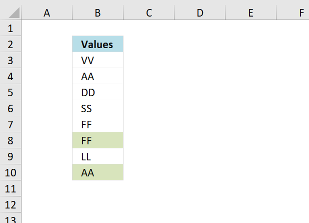
Table of Contents
- How to highlight duplicate values
- Highlight the smallest duplicate number
- Highlight more than once taken course in any given day
- Highlight duplicates in two columns
- Highlight duplicate columns
- Highlight duplicates with same date, week or month
- Highlight duplicate records/rows
- Highlight duplicate values in a cell range
- Highlight duplicates in a filtered Excel Table
1. How to highlight duplicate values
The picture above shows duplicate values in column B, only the second or more duplicates are colored and easily identified.
To sort all duplicates to the bottom of the list for removal, creating a unique distinct list. See this blog post
How to create a unique list using conditional formatting in excel 2007
To color duplicate cells I use conditional formatting in excel. The conditional formatting formula in B3:B11:
1.1 Explaining CF formula
Step 1 - Expanding cell reference
The first argument in the COUNTIF function expands as the CF moves to cells below, this makes it easy to spot duplicate values as their count is 2 or larger.
| Cell | First argument |
| B3 | $B3:$B$3 |
| B4 | $B4:$B$3 |
| B5 | $B5:$B$3 |
Step 2 - Absolute cell reference
The second argument changes to the current cell.
| Cell | Second argument |
| B3 | B3 |
| B4 | B4 |
| B5 | B5 |
Step 3 - Count current value in expanding cell range
COUNTIF($B3:$B$3, B3)
becomes
COUNTIF("VV", "VV")
and returns 1
| Cell | COUNTIF | Evaluates to | Result |
| B3 | COUNTIF($B3:$B$3, B3) | COUNTIF("VV", "VV") | 1 |
| B4 | COUNTIF($B4:$B$3, B4) | COUNTIF({"VV","AA"}, "AA") | 1 |
| B5 | COUNTIF($B5:$B$3, B5) | COUNTIF({"VV","AA","DD"}, "DD") | 1 |
Step 4 - Check if value is larger than 1
COUNTIF($B3:$B$3, B3)>1
becomes
1>1
and returns FALSE. Cell B3 is not highlighted.
1.2 How to highlight duplicate values occurring the second time or more using conditional formatting in Excel
- Select the range (B3:B10)
- Press with left mouse button on the "Home" tab on the ribbon
- Press with left mouse button on "Conditional formatting"
- Press with left mouse button on "New rule..."
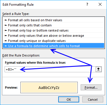
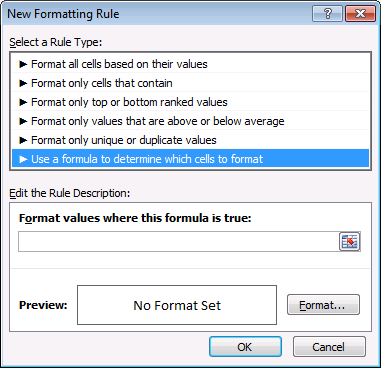
- Press with left mouse button on "Use a formula to determine which cells to format"
- Press with left mouse button on "Format values where this formula is true" window.
- Type COUNTIF($B3:$B$3, $B3)>1
- Press with left mouse button on "Format" button
- Go to tab "Fill"
- Pick a color
- Press with left mouse button on OK button
- Press with left mouse button on OK button again to return to Excel
1.3 Get Excel example file
highlight-duplicates-using-conditional-formatting.xls
(Excel 97-2003 Workbook *.xls)
2. Highlight the smallest duplicate number
Question: How do I highlight the smallest duplicate value in a column using conditional formatting?
Answer:
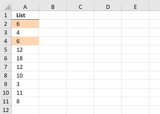
Conditional formatting formula in A2:
2.1 How to apply conditional formatting
- Select cell range
- Go to "Home" tab
- Press with left mouse button on Conditional formatting
- Press with left mouse button on "New Rule.."
- Press with left mouse button on "Use a formula to determine what cells to format"
- Copy the above conditional formatting formula to "Format values where this formula is true:"
- Press with left mouse button on Format button
- Select a formatting you like.
- Press with left mouse button on OK
- Press with left mouse button on OK
2.2 Explaining CF formula in cell A2
Step 1 - Identify duplicates
The COUNTIF function counts values based on a condition or criteria.
COUNTIF($A$2:$A$11, $A$2:$A$11)>1
becomes
COUNTIF({6;4;6;12;18;12;10;3;11;8}, {6;4;6;12;18;12;10;3;11;8})>1
becomes
{2;1;2;2;1;2;1;1;1;1}>1
and returns
{TRUE; FALSE; TRUE; TRUE; FALSE; TRUE; FALSE; FALSE; FALSE; FALSE}.
Step 2 - Extract duplicate numbers
The IF function uses a logical expression in order to determine which argument to return.
IF(COUNTIF($A$2:$A$11, $A$2:$A$11)>1, $A$2:$A$11, "")
becomes
IF({TRUE; FALSE; TRUE; TRUE; FALSE; TRUE; FALSE; FALSE; FALSE; FALSE}, $A$2:$A$11, "")
becomes
IF({TRUE; FALSE; TRUE; TRUE; FALSE; TRUE; FALSE; FALSE; FALSE; FALSE}, {6;4;6;12;18;12;10;3;11;8}, "")
and returns
{6;"";6;12;"";12;"";"";"";""}.
Step 3 - Identify the smallest number in array
The MIN function extracts the minimum value in a cell range or array.
MIN(IF(COUNTIF($A$2:$A$11, $A$2:$A$11)>1, $A$2:$A$11, ""))
becomes
MIN({6;"";6;12;"";12;"";"";"";""})
and returns 6.
Step 4 - Compare smallest number to current cell
MIN(IF(COUNTIF($A$2:$A$11, $A$2:$A$11)>1, $A$2:$A$11, ""))=A2
becomes
6=A2
becomes
6=6
and returns TRUE. Cell A2 is highlighted.
Get Excel *.xls file
highlight-smallest-duplicate-value-in-a-column.xls
3. Highlight more than once taken course in any given day
Answer:
Conditional formatting formula:
Explaining Conditional formatting formula
Step 1 - Count record
The next COUNTIF function counts values based on a condition or criteria.
COUNTIF($A2, $A$2:$A$35)*COUNTIF($B2, $B$2:$B$35)*COUNTIF($C2, $C$2:$C$35)
becomes
{1; 0; 0; 0; 0; 0; 0; 0; 0; 0; 0; 0; 1; 0; 1; 1; 0; 0; 0; 0; 0; 0; 0; 1; 0; 1; 0; 0; 0; 0; 0; 1; 0; 0}*COUNTIF($B2, $B$2:$B$35)*COUNTIF($C2, $C$2:$C$35)
becomes
{1; 0; 0; 0; 0; 0; 0; 0; 0; 0; 0; 0; 1; 0; 1; 1; 0; 0; 0; 0; 0; 0; 0; 1; 0; 1; 0; 0; 0; 0; 0; 1; 0; 0}*{1; 0; 0; 1; 0; 0; 0; 0; 0; 0; 0; 0; 0; 0; 0; 0; 0; 0; 0; 0; 0; 0; 1; 0; 0; 0; 1; 0; 0; 0; 0; 0; 0; 0}*COUNTIF($C2, $C$2:$C$35)
and returns
{1; 0; 0; 0; 0; 0; 0; 0; 0; 0; 0; 0; 1; 0; 1; 1; 0; 0; 0; 0; 0; 0; 0; 1; 0; 1; 0; 0; 0; 0; 0; 1; 0; 0}*{1; 0; 0; 1; 0; 0; 0; 0; 0; 0; 0; 0; 0; 0; 0; 0; 0; 0; 0; 0; 0; 0; 1; 0; 0; 0; 1; 0; 0; 0; 0; 0; 0; 0}*{1; 0; 1; 0; 1; 0; 0; 0; 0; 0; 0; 0; 1; 1; 0; 1; 0; 0; 1; 0; 1; 0; 1; 1; 1; 0; 0; 0; 0; 1; 0; 0; 0; 0}
Step 2 - Multiply arrays
All three arrays must return 1 in order to indicate a row as duplicate, to accomplish this we need to use AND logic. AND logic is performed using the asterisk charcater between arrays, in other words, arrays are multiplied.
COUNTIF($A2, $A$2:$A$35)*COUNTIF($B2, $B$2:$B$35)*COUNTIF($C2, $C$2:$C$35)
becomes
{1; 0; 0; 0; 0; 0; 0; 0; 0; 0; 0; 0; 1; 0; 1; 1; 0; 0; 0; 0; 0; 0; 0; 1; 0; 1; 0; 0; 0; 0; 0; 1; 0; 0}*{1; 0; 0; 1; 0; 0; 0; 0; 0; 0; 0; 0; 0; 0; 0; 0; 0; 0; 0; 0; 0; 0; 1; 0; 0; 0; 1; 0; 0; 0; 0; 0; 0; 0}*{1; 0; 1; 0; 1; 0; 0; 0; 0; 0; 0; 0; 1; 1; 0; 1; 0; 0; 1; 0; 1; 0; 1; 1; 1; 0; 0; 0; 0; 1; 0; 0; 0; 0}
and returns
{1; 0; 0; 0; 0; 0; 0; 0; 0; 0; 0; 0; 0; 0; 0; 0; 0; 0; 0; 0; 0; 0; 0; 0; 0; 0; 0; 0; 0; 0; 0; 0; 0; 0}.
Step 3 - Sum numbers in array
The SUM function adds numbers in a cell range or array and returns a total.
SUM(COUNTIF($A2, $A$2:$A$35)*COUNTIF($B2, $B$2:$B$35)*COUNTIF($C2, $C$2:$C$35))
becomes
SUM({1; 0; 0; 0; 0; 0; 0; 0; 0; 0; 0; 0; 0; 0; 0; 0; 0; 0; 0; 0; 0; 0; 0; 0; 0; 0; 0; 0; 0; 0; 0; 0; 0; 0})
and returns 1.
Step 4 - Check if record is a duplicate
If total is larger than 1 then we know it is a duplicate, the larger than character allows us to compare the total to a given condition, the returned value is a boolean value, TRUE or FALSE.
SUM(COUNTIF($A2, $A$2:$A$35)*COUNTIF($B2, $B$2:$B$35)*COUNTIF($C2, $C$2:$C$35))>1
becomes
1>1 and returns FALSE. Cell A2 is not highlighted.
Get Excel *.xls file
Highlight duplicate online classes using conditional formatting
4. Highlight duplicates in two columns
Question:
Answer:
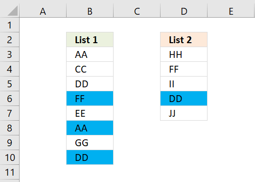
The following animated image shows you two lists in column B and D.
Conditional formatting formula:
How to apply the conditional formatting formulas:
- Select cell range
- Press with left mouse button on "Home" tab on the ribbon
- Press with left mouse button on "Conditional formatting"
- Press with left mouse button on "New rule..."
- Press with left mouse button on "Use a formula to determine which cells to format"
- Press with left mouse button on "Format values where this formula is true" window.
- Type =(COUNTIF($B$3:$B3,B3)+COUNTIF($D$3:$D3,B3))>1
- Press with left mouse button on Format button
- Press with left mouse button on "Fill" tab
- Pick a color
- Press with left mouse button on OK!
- Press with left mouse button on OK!
Explaining formula
Step 1 - Check if current value B3 exists in cell range $B$3:$B3
The first argument in the COUNTIF function is a cell reference that expands downwards.
COUNTIF($B$3:$B3,B3)
| Cell | COUNTIF | Result |
| B3 | COUNTIF($B$3:$B3, B3) | 0 |
| B4 | COUNTIF($B$3:$B4, B4) | 0 |
| B5 | COUNTIF($B$3:$B5, B5) | 0 |
Step 2 - Check if current value B3 exists in cell range $D$3:$D3
The first argument in the COUNTIF function is a cell reference that expands downwards.
COUNTIF($D$3:$D3,B3)
| Cell | COUNTIF | Result |
| B3 | COUNTIF($D$3:$D3, B3) | 0 |
| B4 | COUNTIF($D$3:$D4, B4) | 0 |
| B5 | COUNTIF($D$3:$D5, B5) | 0 |
Step 3 - Add results
COUNTIF($B$3:$B3,B3)+COUNTIF($D$3:$D3,B3)
| Cell | COUNTIF | Result |
| B3 | COUNTIF($B$3:$B3,B3)+COUNTIF($D$3:$D3,B3) | 0 |
| B4 | COUNTIF($B$3:$B4,B4)+COUNTIF($D$3:$D4,B4) | 0 |
| B5 | COUNTIF($B$3:$B5,B5)+COUNTIF($D$3:$D5,B5) | 0 |
Step 4 - Check if result is larger than 1
The parentheses makes sure that the order odf calculatiuon is correct.
(COUNTIF($B$3:$B3,B3)+COUNTIF($D$3:$D3,B3))>1
becomes
(0 (zero) + 0 (zero))>1
0>1
and returns FALSE. Cell B3 is not highlighted.
Get excel *.xlsx file
Highlight duplicates in two lists using conditional formatting.xlsx
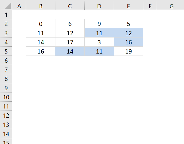
5. Highlight duplicate columns
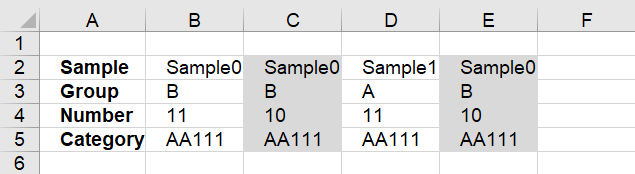
This article describes how to highlight duplicate records arranged into a column each, if you are looking for records entered in a row each then go to this article: Highlight duplicate records. The image above shows one record in each column, cell range B2:E5.
The array formula and conditional formatting formula in this article contain the COUNTIFS function, a function introduced in excel 2007. The COUNTIFS function evaluates conditions on cells across multiple ranges and counts the number of times all are met.
Conditional formatting formula:
How to add conditional formatting formula
- Select cells A1:C30
- Press with left mouse button on "Home" tab
- Press with left mouse button on "Conditional Formatting" button
- Press with left mouse button on "New Rule.."
- Press with left mouse button on "Use a formula to determine which cells to format"
- Type =COUNTIFS($B$2:$E$2, B$2, $B$3:$E$3, B$3, $B$4:$E$4, B$4, $B$5:$E$5, B$5)>1 in "Format values where this formula is TRUE" window.
- Press with left mouse button on "Format.." button
- Press with left mouse button on "Fill" tab
- Select a color for highlighting cells.
- Press with left mouse button on "Ok"
- Press with left mouse button on "Ok"
- Press with left mouse button on "Ok"
Explaining Conditional Formatting Formula in cell B2
Step 1 - Count columns that match the current column
In order to explain how this formula works you need to understand absolute and relative cell references. The dollar sign makes the cell reference locked, however a cell reference has both a column and row part and both may have a dollar sign depending on what you want to happen.
The COUNTIFS function allows you to counts duplicate records, make sure you create a condition for each row in your record. There are four rows in this example, the first argument is $B$2:$E$2 and doesn't change when the conditional formatting moves on to the next column.
The second argument is B$2 and is locked to row 2, however, the column is a relative cell reference (not locked) and changes when the CF moves to next column.
If there are columns that match all four conditions B$2, B$3, B$4 and B$5 then the COUNTIFS function returns the number of rows that match.
COUNTIFS($B$2:$E$2, B$2, $B$3:$E$3, B$3, $B$4:$E$4, B$4, $B$5:$E$5, B$5)
returns 1.
Step 2 - Check if the number is larger than 1
If there is more than one column matching we know the record is a duplicate.
COUNTIFS($B$2:$E$2, B$2, $B$3:$E$3, B$3, $B$4:$E$4, B$4, $B$5:$E$5, B$5)>1
becomes
1>1
and returns FALSE. Cell B2 is not highlighted.
6. Highlight duplicates with same date, week or month
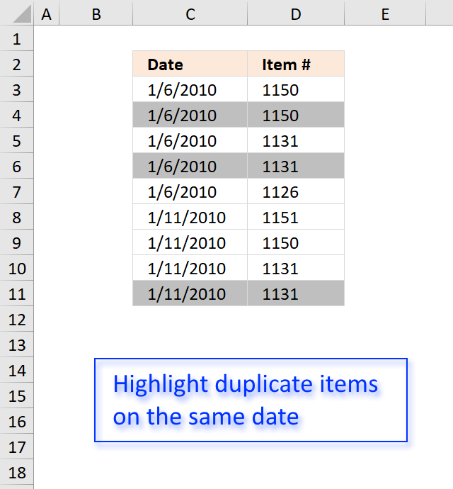
The image above demonstrates a conditional formatting formula that highlights duplicate items based on date. The first instance is not highlighted, only subsequent duplicates are highlighted.
Conditional formatting formula:
6.1 Explaining Conditional formatting formula
Step 1 - Concatenate cell values
The cell references $C3 and $D3 are locked to each column, however, they change when CF move to the next row. The ampersand sign concatenates the values in these cells.
$C3&"-"&$D3
becomes
40184&"-"&1150
and returns
"40184-1150"
Step 2 - Concatenate values using expanding cell references
These cell references expand as the CF moves to cells below, the formula keeps track of previous values so it can detect duplicate values.
$C3:$C$3&"-"&$D3:$D$3
becomes
40184&"-"&1150
and returns
"40184-1150".
Step 3 - Compare concatenated values
The equal sign lets you compare values, the result is always TRUE or FALSE.
$C3&"-"&$D3=$C3:$C$3&"-"&$D3:$D$3
becomes
"40184-1150" = "40184-1150"
and returns TRUE.
Step 4 - Convert boolean values
The SUMPRODUCT function can't work with boolean values, we must convert it (them) to their numerical equivalents. TRUE = 1 and FALSE equals 0 (zero).
--($C3&"-"&$D3=$C3:$C$3&"-"&$D3:$D$3)
becomes
--(TRUE)
and returns 1.
Step 5 - Sum values
The SUMPRODUCT function sums the values in the array in this step.
SUMPRODUCT(--($C3&"-"&$D3=$C3:$C$3&"-"&$D3:$D$3))
becomes
SUMPRODUCT(1)
and returns 1.
Step 6 - Check if duplicate
This steps checks if the sum is larger than 1, if it is then TRUE is returned and the cell is highlighted.
SUMPRODUCT(--($C3&"-"&$D3=$C3:$C$3&"-"&$D3:$D$3))>1
becomes
1>1
and returns FALSE. Cell C3 is not highlighted.
6.2 Get Excel *.xlsx file
Highlight-duplicates-within-same-date-week-month-year.xlsx
6.3 Highlight duplicates on same week

Conditional formatting formula:
6.4 Highlight duplicates on same month

Conditional formatting formula:
Get excel sample file for this article.
Highlight-duplicates-within-same-date-week-month-year.xls
(Excel 97-2003 Workbook *.xls)
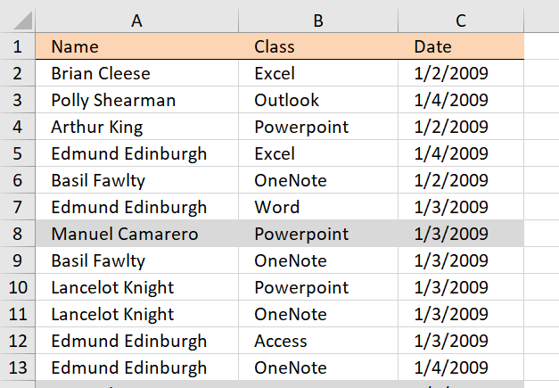
7. Highlight duplicate records/rows
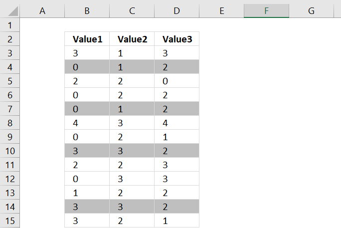
This section shows you how to easily identify duplicate rows or records in a list.
7.1. Conditional Formatting formula - Excel 2007 and later versions
Conditional formatting formula:
7.2. Conditional Formatting formula - Excel 2003 and previous versions
The COUNTIFS function was introduced in Excel 2007, here is a formula for previous versions:
7.3. How to create a conditional formatting formula
- Select the cell range you want to highlight duplicate rows for.
- Go to the "Home" tab on the ribbon.
- Press with left mouse button on the "Conditional Formatting" button. A popup menu appears.
- Press with left mouse button on "New Rule.." on the popup menu.
- Press with left mouse button on "Use a formula to determine which cells to format", see the image below.
- Type =COUNTIFS($B$3:$B$15,$B3,$C$3:$C$15,$C3,$D$3:$D$15,$D3)>1 in "Format values where this formula is TRUE" window.
- Press with left mouse button on "Format.." button
- Press with left mouse button on "Fill" tab
- Select a color for highlighting cells.
- Press with left mouse button on "Ok"
- Press with left mouse button on "Ok"
- Press with left mouse button on "Ok"
7.4. How the conditional formatting formula works
Step 1 - Count rows that match the current row
The COUNTIFS function allows you to counts duplicate records, make sure you create a condition for each column in your record. There are three columns in this example, the first argument is $B$3:$B$15 and doesn't change when the conditional formatting moves on to the next row.
The second argument is $B3 and is locked to column B, however, the row is a relative cell reference (not locked) and changes when the CF moves to the next row.
If there are rows that match all three conditions $B3, $C3 and $D3 the COUNTIFS function returns the number of rows that match.
COUNTIFS($B$3:$B$15, $B3, $C$3:$C$15, $C3, $D$3:$D$15, $D3)
returns 1 because the first row is counted as well.
Step 2 - Check if the number is larger than 1
If there is more than one row matching we know the record is a duplicate.
COUNTIFS($B$3:$B$15, $B3, $C$3:$C$15, $C3, $D$3:$D$15, $D3)>1
becomes
1>1
and returns FALSE. Cell B3 is not highlighted.
7.5. Do not highlight the first duplicate
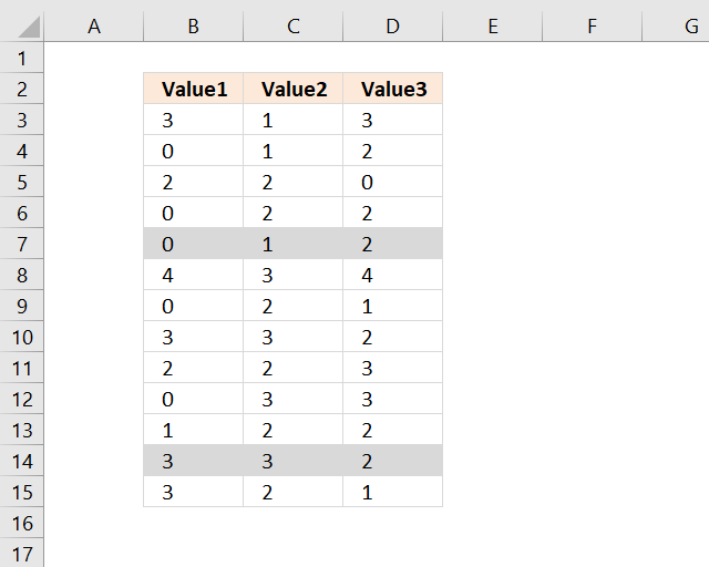
The following CF formula highlights duplicates except the first instance, see image above.
Recommended blog post
Automatically filter unique distinct row records
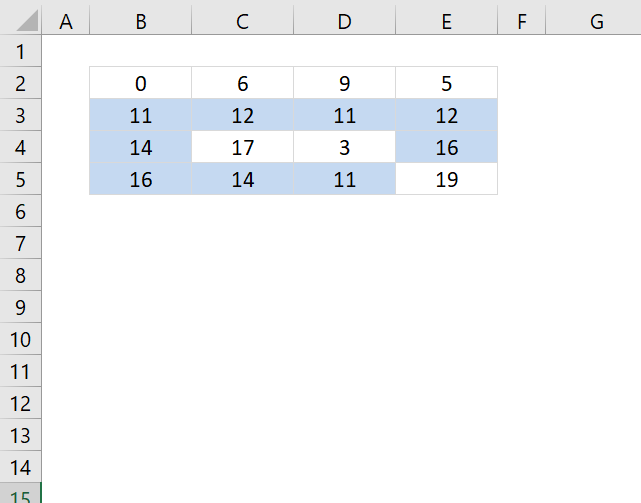
8. Highlight duplicate values in a cell range
The following conditional formula highlights only the second instance or more of a value in a cell range.
Conditional formatting formula:
How to apply conditional formatting
- Select your range B2:E5.
- Go to "Home" tab
- Press with left mouse button on Conditional formatting
- Press with left mouse button on "New Rule.."
- Press with left mouse button on "Use a formula to determine what cells to format"
- Copy and paste the above conditional formatting formula to "Format values where this formula is true:"
- Press with left mouse button on Format button
- Select a formatting you like. For example, cells filled with yellow.
- Press with left mouse button on OK
- Press with left mouse button on OK
8.1 Explaining CF formula in cell B2
There are two parts in this formula, one part determines if a value is a duplicate in the first column. The second part of the formula determines if a value is a duplicate in the remaining columns.
The reason the formula looks like this is because of the order of how Excel calculates cells.
IF(logical_expression, first_part, second_part)
Step 1 - Check if first column is being evaluated
The COLUMNS function counts columns in a cell reference. $A$1:A1 is an expanding cell reference, it grows because A1 is a relative cell reference that changes between cells.
COLUMNS($A$1:A1)=1
becomes
1=1 and returns TRUE.
Step 2 - Count cells based on a condition
The IF function changes the calculation based on the logical expression in the first argument. The second argument is calculated if the logical expression returns TRUE, the third argument is calculated if the logical expression returns FALSE.
The COUNTIF function makes sure that duplicates are not highlighted, only the first instance of each value. However this works only in the first column, the remaining columns need a different formula in order to do correct calculations.
IF(COLUMNS($A$1:A1)=1,COUNTIF($B$2:B2,B2),COUNTIF($B$2:B2,B2)+COUNTIF(OFFSET($B$2:$E$5,,,4,COLUMNS($A$1:A1)-1),B2))>1
becomes
IF(TRUE,COUNTIF($B$2:B2,B2),...)>1
becomes
IF(TRUE,COUNTIF(0,0),...)>1
becomes
1>1
and returns FALSE. Cell B2 is not highlighted.
Step 3 - Calculations in remaining columns
If we move to cell C2 the IF function behaves differently.
IF(COLUMNS($A$1:B1)=1, COUNTIF($B$2:C2, C2), COUNTIF($B$2:C2, C2)+COUNTIF(OFFSET($B$2:$E$5, ,,4, COLUMNS($A$1:B1)-1), B2))>1
becomes
IF(2=1, COUNTIF($B$2:C2, C2),COUNTIF($B$2:C2, C2)+COUNTIF(OFFSET($B$2:$E$5, , , 4, COLUMNS($A$1:B1)-1), C2))>1
becomes
IF(FALSE, COUNTIF($B$2:C2, C2), COUNTIF($B$2:C2, C2)+COUNTIF(OFFSET($B$2:$E$5, , , 4, COLUMNS($A$1:B1)-1), C2))>1
becomes
IF(FALSE, COUNTIF($B$2:C2, C2), COUNTIF({0,6}, 6)+COUNTIF(OFFSET($B$2:$E$5, , , 4, COLUMNS($A$1:B1)-1), C2))>1
The OFFSET function returns an expanding cell reference that grows as the CF moves from column to column.
IF(FALSE, COUNTIF($B$2:C2, C2), 1+COUNTIF(OFFSET($B$2:$E$5, , , 4, 1), C2))>1
becomes
IF(FALSE, COUNTIF($B$2:C2, C2), 1+COUNTIF($B$2:$B$5, C2))>1
becomes
IF(FALSE, COUNTIF($B$2:C2, C2), 1+COUNTIF({0;11;14;16},6))>1
becomes
IF(FALSE, COUNTIF($B$2:C2, C2), 1+0)>1
becomes
1>1 and returns FALSE. Cell C2 is not highlighted.
8.2 Highlight all duplicates
To highlight all duplicates is much easier, the formula simply counts how many times the current value exists in the cell range.
Get excel *.xlsx file
highlight duplicate values in a range.xlsx
9. Highlight duplicates in a filtered Excel Table

The image above demonstrates a conditional formatting formula applied to an Excel Table containing random data. The Excel Table has been filtered to show only records for January 2012.
There is a built-in function in Excel that lets you highlight duplicates, however, that won't work properly if you have filtered the data.
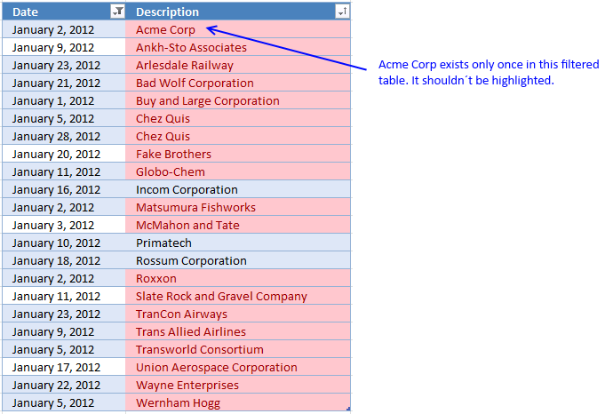
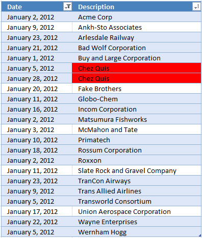
The image above shows the built-in tool highlighting duplicate items. But one item exists only once in the filtered data, however, it is highlighted as a duplicate.
The reason is that there is another item not showing in the filtered table. You need to rely on a custom conditional formatting formula if you want it to compare only filtered visible values.
9.1 Build an Excel Table
The reason I am using an Excel Table is that the conditional formatting adjusts automatically if you add or delete records. It also uses structured references so there is no need to change cell references in the formula.
The disadvantage is that you have to use the INDIRECT function each time you reference the Excel Table in the CF formula, it is not a big deal but it is worth noting.
- Select any cell in your data set.
- Press short cut keys CTRL + T to open the "Create Table" dialog box.

- Enable the checkbox if the columns in the data set have header names.
- Press with left mouse button on OK button to apply.
9.2 Create a new conditional formatting rule
- Select table column "Description".
- Go to the "Home" tab on the ribbon.
- Press with left mouse button on the "Conditional formatting" button.
- Press with left mouse button on "New Rule..".
- Press with left mouse button on "Use a formula to determine which cells to format".
- Copy this conditional formatting formula:
=SUM(COUNTIF(INDIRECT("Table2[@Description]"), IF(SUBTOTAL(3, OFFSET(INDIRECT("Table2[Description]"), MATCH(ROW(INDIRECT("Table2[Description]")), ROW(INDIRECT("Table2[Description]")))-1, 0, 1)), INDIRECT("Table2[Description]"), "")))>1
- Paste to "Format values where this formula is true:". I will explain the formula later in this article.
- Press with left mouse button on the "Format..." button.
- Go to tab "Fill".

- Pick a color.
- Press with left mouse button on OK button.
- Press with left mouse button on OK button again.
9.3 Explaining CF formula in cell C211
This Conditional Formatting formula highlights cells that have a duplicate in a filtered Excel Table, note that it will not be highlighted if a duplicate exists outside the filtered values (not visible).
Step 1 - Create an array from 1 to n
The INDIRECT function makes it possible to use a reference to an Excel Table inside a Conditional Formatting formula. This article explains it in greater detail: How to use an Excel Table name in Data Validation Lists and Conditional Formatting formulas
The ROW function converts a cell reference to the corresponding row numbers which is useful when you want to create an array.
The MATCH function is utilized in this example to create an array that contains a sequence that begins with 1 and increments with one up to the number of values in the array.
MATCH(ROW(INDIRECT("Table2[Description]")), ROW(INDIRECT("Table2[Description]"))
becomes
MATCH(ROW(C206:C227), ROW(C206:C227))
becomes
MATCH({3; 4; ... 383; 384}, {3; 4; ... 383; 384})
and returns
{1; 2; 3; ... 380; 381}.
The Excel Table has 381 records and the size of the array matches that number.
Step 2 - Modify array
This workaround makes it possible to use an array of values in a SUBTOTAL function, the OFFSET function splits the array into smaller arrays with only one value in each array.
OFFSET(reference,rows,columns,[height],[width])
It returns error values, however, the SUBTOTAL function can calculate these values anyway.
OFFSET(INDIRECT("Table2[Description]"), MATCH(ROW(INDIRECT("Table2[Description]")), ROW(INDIRECT("Table2[Description]")))-1, 0, 1)
becomes
OFFSET(INDIRECT("Table2[Description]"), {1; 2; 3; ... 380; 381}-1, 0, 1)
becomes
{0; 1; 2; ... ; 379; 380}
and returns
{#VALUE!; #VALUE!; #VALUE!; ... ; #VALUE!; #VALUE!}
Step 3 - Identify visible values
The first argument in the SUBTOTAL function is 3 and represents the COUNTA function meaning it will count cells that are not empty.
The SUBTOTAL function will actually return an array with this setup which is very handy in this situation.
SUBTOTAL(3, OFFSET(INDIRECT("Table2[Description]"), MATCH(ROW(INDIRECT("Table2[Description]")), ROW(INDIRECT("Table2[Description]")))-1, 0, 1))
becomes
SUBTOTAL(3, {#VALUE!; #VALUE!; #VALUE!; ... ; #VALUE!; #VALUE!})
and returns {0; 0; 0; ... ; 0; 0}. 0 (zero) represents a hidden value and 1 is visible.
Step 4 - Create an array containing visible values
The IF function replaces 0 (zero) with nothing "" and 1 with the actual corresponding value.
IF(SUBTOTAL(3, OFFSET(INDIRECT("Table2[Description]"), MATCH(ROW(INDIRECT("Table2[Description]")), ROW(INDIRECT("Table2[Description]")))-1, 0, 1)), INDIRECT("Table2[Description]"), "")
becomes
IF({0; 0; 0; ... ; 0; 0}, INDIRECT("Table2[Description]"), "")
and returns {""; ""; ""; ... ; ""; ""}.
Step 5 - Check the number of times the current value exists across visible values
The COUNTIF function will return an array with this setup which we then can use to calculate a total. The reason we don't change the arguments with each other is that the range argument will not accept an array based on calculations.
COUNTIF(range, criteria)
COUNTIF(INDIRECT("Table2[@Description]"), IF(SUBTOTAL(3, OFFSET(INDIRECT("Table2[Description]"), MATCH(ROW(INDIRECT("Table2[Description]")), ROW(INDIRECT("Table2[Description]")))-1, 0, 1)), INDIRECT("Table2[Description]"), ""))
becomes
COUNTIF(INDIRECT("Table2[@Description]"), {""; ""; ""; ... ; ""; ""})
becomes
COUNTIF("Chez Quiz", {""; ""; ""; ... ; ""; ""})
and returns {0; 0; 0; ... ; 0; 0}. The entire array is not shown, however, it contains a few 1's as well.
Step 6 - Calculate a total
The SUM function adds all numbers in the array and returns a total.
SUM(COUNTIF(INDIRECT("Table2[@Description]"), IF(SUBTOTAL(3, OFFSET(INDIRECT("Table2[Description]"), MATCH(ROW(INDIRECT("Table2[Description]")), ROW(INDIRECT("Table2[Description]")))-1, 0, 1)), INDIRECT("Table2[Description]"), "")))
becomes
SUM({0; 0; 0; ... ; 0; 0})
and returns 2.
Step 7 - Check if value is larger than 1
The > larger than character is a logical operator that lets you compare values, it will return a boolean value TRUE or FALSE based on the outcome. The Conditional Formatting formula uses the boolean function to determine if the cell values should be highlighted or not.
SUM(COUNTIF(INDIRECT("Table2[@Description]"), IF(SUBTOTAL(3, OFFSET(INDIRECT("Table2[Description]"), MATCH(ROW(INDIRECT("Table2[Description]")), ROW(INDIRECT("Table2[Description]")))-1, 0, 1)), INDIRECT("Table2[Description]"), "")))>1
becomes
2>1
and returns True. Cell C211 is highlighted.
Recommended reading
Built-in conditional formatting
Data Bars Color scales IconsHighlight cells rule
Highlight cells containing stringHighlight a date occuring
Conditional Formatting Basics
Highlight unique/duplicates
Top bottom rules
Highlight top 10 valuesHighlight top 10 % values
Highlight above average values
Basic CF formulas
Working with Conditional Formatting formulasFind numbers in close proximity to a given number
Highlight empty cells
Highlight text values
Search using CF
Highlight records – multiple criteria [OR logic]Highlight records [AND logic]
Highlight records containing text strings (AND Logic)
Highlight lookup values
Unique distinct
How to highlight unique distinct valuesHighlight unique values and unique distinct values in a cell range
Highlight unique values in a filtered Excel table
Highlight unique distinct records
Duplicates
How to highlight duplicate valuesHighlight duplicates in two columns
Highlight duplicate values in a cell range
Highlight smallest duplicate number
Highlight more than once taken course in any given day
Highlight duplicates with same date, week or month
Highlight duplicate records
Highlight duplicate columns
Highlight duplicates in a filtered Excel Table
Compare
Highlight missing values between to columnsCompare two columns and highlight values in common
Compare two lists of data: Highlight common records
Compare tables: Highlight records not in both tables
How to highlight differences and common values in lists
Compare two columns and highlight differences
Min max
Highlight smallest duplicate numberHow to highlight MAX and MIN value based on month
Highlight closest number
Dates
Advanced Date Highlighting Techniques in ExcelHow to highlight MAX and MIN value based on month
Highlight odd/even months
Highlight overlapping date ranges using conditional formatting
Highlight records based on overlapping date ranges and a condition
Highlight date ranges overlapping selected record [VBA]
How to highlight weekends [Conditional Formatting]
How to highlight dates based on day of week
Highlight current date
Misc
Highlight every other rowDynamic formatting
Advanced Techniques for Conditional Formatting
Highlight cells based on ranges
Highlight opposite numbers
Highlight cells based on coordinates
Excel categories
19 Responses to “How to highlight duplicate values”
Leave a Reply
How to comment
How to add a formula to your comment
<code>Insert your formula here.</code>
Convert less than and larger than signs
Use html character entities instead of less than and larger than signs.
< becomes < and > becomes >
How to add VBA code to your comment
[vb 1="vbnet" language=","]
Put your VBA code here.
[/vb]
How to add a picture to your comment:
Upload picture to postimage.org or imgur
Paste image link to your comment.
For those wanting to know how to do this in versions of Excel prior to XL2007, here is the Conditional Formatting formula to use. Select the cells in Columns A, B and C from Row 1 down to the last row you want to conditionally format and use this Conditional Formatting formula...
.
.
=SUMPRODUCT(--($A$1:$A$30&"X"&$B$1:$B$30&"X"&$C$1:$C$30=$A1&"X"&$B1&"X"&$C1))>1
.
.
Those embedded X's just need to be a character that is guaranteed not to be in any of the cells being conditionally formatted. These characters ensure no accidental matches occur during the concatenations; for example, without them, an accidental match could occur like this...
"12"&"3"&"4" = "1"&"23"&"4"
both equating to "1234" meaning the equality check would be true; with the X's in place, you get this...
"12"&"X"&"3"&"X"&"4" = "1"&"X"&"23"&"X"&"4"
with the first equating to "12X3X4" and the second equating to "1X23X4" and the equality check would be false.
Here is another conditional formatting formula, excel 2003:
=SUMPRODUCT(COUNTIF($A1, $A$1:$A$30)*COUNTIF($B1, $B$1:$B$30)*COUNTIF($C1, $C$1:$C$30))>1
When you modiy to move to anu other column apart from 'A' the the first instance of the duplicate also highlights.
David Gordon,
You are right, I believe the new formula I have added to this post is more useful.
Thanks for commenting!
this formula is not working for me.....
Deepak,
what does your formula look like?
Remember, you must understand how relative and absolute cell references work.
[...] Here is a post where I use this technique: Highlight duplicate rows [...]
Love you for this formula. Thank you for posting....
Mohasin,
Thank you for commenting!
[…] has some incredible tools for highlighting cells, rows, dates, comparing data and even series in line charts. A technique using the secondary […]
Thank you for the great post! I had spent almost a full day searching for how to highlight duplicates in a filtered list. But I have one further question. I am filtering this based on duplicate dollar amounts. How could I add in a part of the function to only highlight the duplicate amounts over $900 in the filtered table?
Oscar, Our company requires all employees to take 30 Mandatory Annual Courses. I have been tasked with streamlining the class schedule. I created in access a query that pulls all courses and personnel that are due to take these courses within 45 days. I export to excel and then sort on the courses and then the supervisor. After that I subtotal and get 30 subtotals for each course. The number of records in each subtotal course varies.
My max class size per course is 14 and the max number of people per supervisor is 5. How can I
Oscar,
My company requires all employees to take Mandatory Annual Courses.
We have 30 courses.
I have been tasked with streamlining the class schedule. I have all courses listed along with the names of the personnel along with their department and supervisor. I sort by class name and then by supervisor. I then subtotal and get 30 separate subtotals per course. Number of records in each subtotal will vary.
My max class size is 14 and the most I can pull from each supervisor per class per course is 5.
How can I create a formula for each subtotal that will determine the number of classes based on a max class size of 14 and then assign the max number of personnel per class per supervisor of 5.
Example: Course Name: Active Shooter
42 people need to attend this class, There are 6 supervisors for these 42 people. On the surface it looks like 3 classes,however one supervisor has 16 people which would exceed the max per class of 5.
Any help is appreciated.
Regards
Gene Haines
Gene Haines,
My max class size is 14 and the most I can pull from each supervisor per class per course is 5. 42 people need to attend this class, there are 6 supervisors for these 42 people.
You only have 6 supervisors, don't you need more supervisors per class per course if your class is 42? If each supervisor has 5 people you get 6x5 = 30 people.
This criteria is not met if your class is above 30 people?
Hello, this formula works great, I am wondering if I can change it slightly for what I need.
I have rows of lists, 6 in each row. They are all names. The names will be in different order, but I want to not have duplicates of the same lists. I cannot fully sort them as the first name is unique, and needs to be in that spot. I will give you and example:
John Bill James Ron Joe Mike
Bill John James Joe Ron Mike
James Bill John Joe Mike Ron
All three of these list are the same, but when they are in a different order, this conditional formatting does not show them as duplicates. Any suggestions?
Thank you in advance,
Marsh
exactly what i was searching for. unfortunately way more cumbersome than i hoped, but a solution nevertheless. thanks a lot!
Hi,
I'm trying to find a way to highlight cells with text/number (column B) if reoccurred 3 times or more within the last 3 days (dates in column A)
I hope someone can help
Hello,
I'm doing this for a spreadsheet where I don't want a blank cell (in the second column) to match with another blank cell. How can I modify the formula accordingly? For instance, in my work I drag down the dates in column A before entering the rest of the data. I'm looking for a match between column A&E between rows. But at the moment it does this, but also highlights all the prepped rows at the end where I've dragged down the date. I want it not to consider the same date in A and a blank in E to be a match with another same date A and blank E.
Thanks!
Feliz tarde, el archivo de trabajo ya no está disponible. Podría volver a colocarlo??