Working with Conditional Formatting formulas
In this post I am going to try to explain formula basics in conditional formatting. It is really good if you have some knowledge about absolute and relative cell references but it is not necessary. I think the examples shown here explains a lot when it comes to cell referencing.
Conditional formatting is extremely volatile and is even recalcualted every time you scroll the sheet. Remember this if you already work with cpu instensive workbooks.
When creating conditional formatting formulas, I think you will be using mostly comparison operators (=<>) but you can also use functions. Functions I recommend: COUNTIF(), COUNTIFS(), SEARCH(), FIND()
Table of Contents
How to create conditional formatting
- Select a cell range where you want to apply conditional formatting.
- Go to "Home" tab
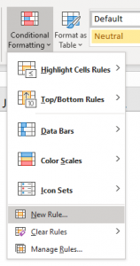
- Press with left mouse button on "Conditional Formatting" button
- Press with left mouse button on "New Rule.."
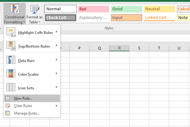
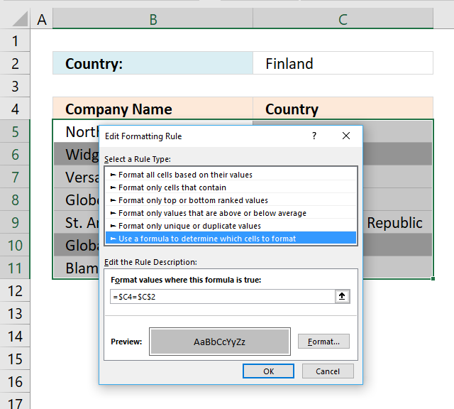
- Press with left mouse button on "Use a formula to determine which cells to format:"
- Type formula in "Format values where this formula is true:"
- Press with left mouse button on "Format..." button

- Choose formatting

- Press with left mouse button on OK
- Press with left mouse button on OK
Your first conditional formatting formula
Let´s create your first conditional formatting formula. Here is a table with some random data.

Select cell range A1: D21 Repeat above steps and use this formula:
I used a grey formatting color.

A1 is a cell reference to the uppermost, leftmost cell in your selected cell range. Relative cell reference changes depending on which cell is calculated. Using cell A1 in the conditional formatting formula, applied to cell range A1:D21 makes it compare each cell in the cell range to the value "Poland".
Example 1,
In cell A1:
Conditional formatting formula:
=A1="Poland"
becomes
="Company Name"="Poland"
and returns False. Cell A1 is NOT formatted.
Example 2,
In cell B9:
The conditional formatting formula changes automatically to:
=B9="Poland"
becomes
="Poland"="Poland"
and returns True. Cell B9 is formatted.
Format entire row
Let´s say you are interested in highlighting rows where cell value in column B is equal to "Poland".
Conditional formatting formula:

Example 1,
In cell A1:
Conditional formatting formula:
=$B1="Poland"
becomes
="Country"="Poland"
and returns False. Cell A1 is NOT formatted.
Example 2,
In cell A9:
The conditional formatting formula changes automatically to:
=$B9="Poland"
becomes
="Poland"="Poland"
and returns True. Cell A9 is formatted. In fact, the entire row is highlighted. The $ makes the cell reference "locked" to column B.
Compare a cell value to a column
Every time you want to change the value you are searching for you must first select the cell range, change the conditional formatting formula and then press OK. Boring repetitive actions, but if you change the value in the conditional formatting formula to an absolute cell reference things start to become more useful. Let me show you how:

Conditional formatting formula:
=$B4=$B$1
Cell value in B1 is compared to every cell value in column B. If the conditional formatting formula returns TRUE the entire row is highlighted.
With the same technique you can highlight an entire column, example: Search with conditional formatting
Column to column comparisons
Now I am going to show you how to use conditional formatting to easily identify companies with increasing sales.

Highlight increasing sales years
Conditional formatting formula:
=C2>B2
Highlight decreasing sales years
Conditional formatting formula:
=C2<B2
Remember to use the uppermost leftmost cell reference in the selected cell range when constructing conditional formatting formulas. In this example, I have applied CF to cell range C2:E21 and C2 is the first cell in that range to be compared to the previous year.
Highlight unique rows
This example demonstrates how to highlight unique distinct rows.

Conditional formatting formula:
Here is an explanation of how the countifs function works.
2. Highlight text values
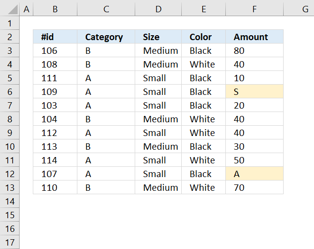
The conditional formatting formula applied to cell range F3:F13 highlights all cells containing text. Here is how I did it:
- Select cell range F3:F13
- Go to tab "Home" on the ribbon
- Press with mouse on "Conditional Formatting" button
- Press with mouse on "New Rule.."
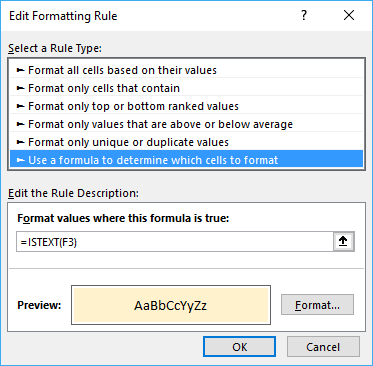
- Select "Use a formula to determine which cells to format"
- Type =ISTEXT(F3) in field "Format values where this formula is true:"
- Then press with left mouse button on "Format..." button
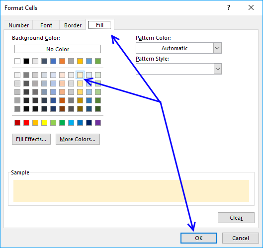
- Go to tab "Fill"
- Pick a color
- Press with left mouse button on OK button
- Press with left mouse button on OK button to return to Excel.
Explaining conditional formatting formula
Why =ISTEXT(F3)? The cell range we want to highlight empty cells in is F3:F13 so the cell we must highlight first is the cell in the cell range.
Cell reference F3 is a relative cell reference and changes in the cell range we want to format, see picture below.
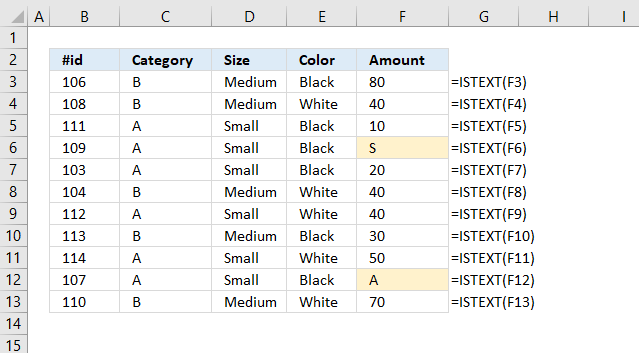
If ISTEXT(F3) returns TRUE the cell is highlighted and FALSE returns nothing. Check out more IS-functions in the Information category.
Get Excel *.xlsx file
3. Highlight empty cells
![]()
The image above shows a data set containing a few random blanks. A conditional formatting formula highlights the empty cells yellow.
Conditional formatting formula:
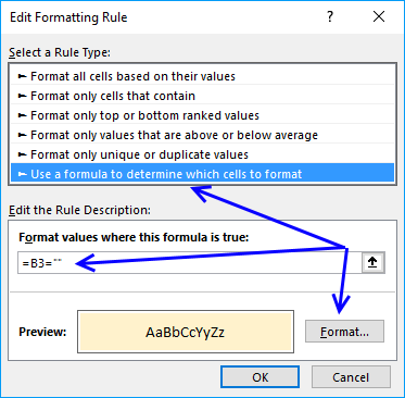
3.1 Explaining conditional formatting formula
Step 1 - Specify relative cell reference
![]()
The image above shows what the CF formula looks like in each cell, the actual cells do not contain this formula.
The cell range we want to highlight empty cells in is B3:F13 so the cell we must highlight first is the cell in the upper left corner in order to highlight the correct cells.
Cell B3 is a relative cell reference and changes in the cell range we want to format. If we started with B4 cell B3 will be highlighted if cell B4 is empty and we don't want that. We want to highlight the empty cell.
Step 2 - Create a logical expression
The equal sign is a logical operator and the result is a boolean value TRUE or FALSE.
B3=""
becomes
106=""
and returns FALSE. Cell B3 is not highlighted.
3.2 How to apply conditional formatting
The conditional formatting formula applied to cell range B3:F15 highlights all blank cells yellow. Here is how I did it:
- Select cell range B3:F13.
- Go to tab "Home" on the ribbon.
- Press with mouse on the "Conditional Formatting" button.
- Press with mouse on "New Rule..".
- Select "Use a formula to determine which cells to format".
- Type =B3="" in field "Format values where this formula is true:".
- Then press with left mouse button on "Format..." button.
- Go to tab "Fill".
- Pick a color.
- Press with left mouse button on OK button.
- Press with left mouse button on OK button to return to Excel.
3.3 Formulas returning nothing.

Note, a cell is conditionally formatted if it contains a formula that returns nothing "". The cell is not highlighted if the formula returns a value.
The image above demonstrates a formula in cell C13 that returns nothing "", the cell is highlighted. Cell C13 is selected and the formula is displayed in the formula bar.
3.4 Cells with hidden values

The image above shows an empty cell E3 but it is not highlighted, cell E3 is actually not empty, it is only formatted to hide values.

Go to the "Format Cells" dialog box to inspect cells that should have been highlighted. The dialog box above shows cell E3 with a custom cell formatting. ;;; hides all values in a cell, select category: General to show the value again.
3.5 Highlight error cells

The image above demonstrates a conditional formatting formula that highlights cells containing an error.
Conditional formatting formula:
3.5.1 Explaining formula
Step 1 - Specify cell reference
The conditional formatting formula is applied to cell range B3:F13, the cell reference must point to the upper left cell which is cell B3 in this example.
B3 returns 106.
Cell reference B3 is a relative cell reference, it changes accordingly when the parser goes to the next cell. It is possible to use absolute cell references, however, this will not work in this example.
Step 2 - Identify error value
The ISERROR function returns TRUE if the value is an error value.
ISERROR(value)
ISERROR(B3)
becomes
ISERROR(106)
and returns FALSE. Cell B3 is not highlighted.
Get Excel *.xlsx file
4. Find numbers in close proximity to a given number
This article demonstrates how to apply Conditional Formatting formula to a cell range, it finds cells that are in close proximity to a given set of numbers based on a range value.
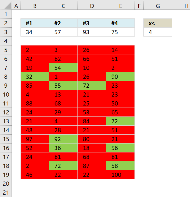
The image above shows 4 values in cell range B3:E3, the range number is in cell G3. A conditional formatting formula highlights cells in cell range B5:E19 that contain a number that is near at least one of the four values in cell range B3:E3.
For example, the image above shows 34, 57, 93 and 75. The range is 4. If 2 which is the cell value in B5 is in proximity with 34, 57 , 93 or 75 then cell B5 is highlighted green.
Number 34 has a higher bound 34 +4 = 38 and a lower bound of 34 - 4 = 30. 2 is not between 30 and 38.
Number 57 has a higher bound 57 + 4 = 61 and a lower bound of 57 - 4 = 53. 2 is not between 53 and 61.
Number 93 has a higher bound 93+ 4 = 97 and a lower bound of 93 - 4 = 89. 2 is not between 89 and 97.
Number 75 has a higher bound 75+ 4 = 79 and a lower bound of 75 - 4 = 71. 2 is not between 71 and 79. Cell B5 is highlighted red.
This article is inspired by a question found here.
Is this possible?Something like Abs(any number in array-any number in row < 4, Highlight green, highlight red) I think I have to utilize index or match functions but I'm having difficulty.
Conditional formatting formulas
Green:
Red:
You can also use this formula for highlighting cells red.
How to apply conditional formatting formulas
- Select cell range (B5:E19)
- Go to tab "Home" on the ribbon.
- Press with mouse on the "Conditional formatting" button.
- Press with left mouse button on "New Rule...".
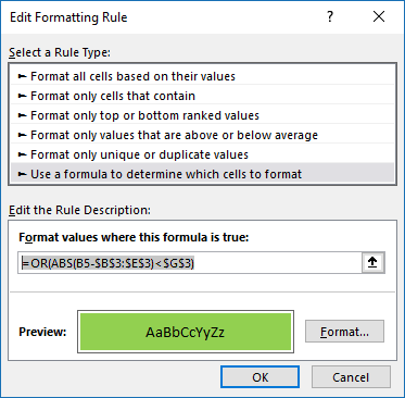
- Select "Use a formula to determine which cells to format".
- Paste =OR(ABS(B5-$B$3:$E$3)<$G$3) to Format values where this is TRUE:
- Press with left mouse button on "Format" button
- Go to tab "Fill"
- Select a color
- Press with left mouse button on ok
- press with left mouse button on ok
Explaining "green" formula in cell A4
Step 1 - Subtract value in cell B5 with array of values specified in $B$3:$E$3
B5-$B$3:$E$3
becomes
2-{34, 57, 93, 75}
and returns
{-32, -55, -91, -73}
Step 2 - Return the absolute value of a number
The ABS function removes the minus sign from a number.
ABS(B5-$B$3:$E$3)
becomes
ABS({-32, -55, -91, -73})
and returns
{32, 55, 91, 73}
Step 3 - Check if values are less than value in cell G3
The less than character < lets you check if a number is less than another number.
ABS(B5-$B$3:$E$3)<$G$3
becomes
{32, 55, 91, 73}<4
and returns
{FALSE, FALSE, FALSE, FALSE}
This means that the value in cell B5 is not in proximity within any of the numbers in cell range B3:E3.
Step 4 - Return FALSE only if all values are FALSE
The OR function returns TRUE if at least one of the boolean values in the array is TRUE and FALSE if all values are FALSE.
OR(ABS(A4-$A$2:$D$2)<$F$1)
becomes
OR({FALSE, FALSE, FALSE, FALSE})
and returns FALSE. Cell B5 is not highlighted green.
5. Highlight records - multiple criteria - OR logic
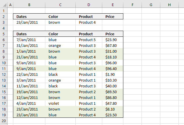
The image above shows you how to highlight rows with multiple criteria using OR logic. The criteria are found in row 3.
A row is highlighted if:
- Date criterion is found in column B or
- Color criterion is found in column C or
- Product criterion is found in column D or
- Price criterion is found in column E
Conditional formatting formula:
Explaining formula in cell D11
Step 1 - Understand how relative and absolute cell references work
In cell B6 the formula is: =SUMPRODUCT(($B$3=$B6)+($C$3=$C6)+($D$3=$D6)+($E$3=$E6))
and in cell D11 the formula has changed to =SUMPRODUCT(($B$3=$B11)+($C$3=$C11)+($D$3=$D11)+($E$3=$E11))
Read more about relative and absolute cell references
Step 2 - OR logic is created using + signs between criteria
=SUMPRODUCT(($B$3=$B11)+($C$3=$C11)+($D$3=$D11)+($E$3=$E11))
becomes
=SUMPRODUCT((40566=40552)+("brown"="blue")+("Product 4"="Product 4")+(""=96,40))
becomes
=SUMPRODUCT(FALSE+FALSE+TRUE+FALSE)
becomes
=SUMPRODUCT(0+0+1+0) and returns 1. (TRUE)
Cell D11 is highlighted
How to apply conditional formatting formula
Make sure you adjust cell references to your excel sheet.
-
- Select cells B6:E27
- Press with left mouse button on "Home" tab
- Press with left mouse button on "Conditional Formatting" button
- Press with left mouse button on "New Rule.."
- Press with left mouse button on "Use a formula to determine which cells to format"
- Type =SUMPRODUCT(($B$3=$B6)+($C$3=$C6)+($D$3=$D6)+($E$3=$E6)) in "Format values where this formula is TRUE" window.
- Press with left mouse button on "Format.." button
- Press with left mouse button on "Fill" tab
- Select a color for highlighted cells.
- Press with left mouse button on "Ok"
- Press with left mouse button on "Ok"
- Press with left mouse button on "Ok"
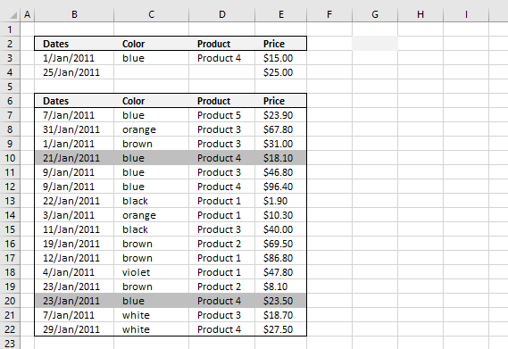
Date range and price range criteria
Let's set up a new sheet with a date range as a criterion and a price range as another criterion.
A row is highlighted if:
- A date is smaller or equal to cell B4 and the same date is larger or equal to cell B3 or
- Color criterion is found in column C or
- Product criterion is found in column D or
- A price is smaller or equal to cell E4 and the same price is larger or equal to cell E3

Conditional formatting formula:
How to apply conditional formatting formula
Make sure you adjust cell references to your excel sheet.
- Select cells B6:E27
- Press with left mouse button on "Home" tab
- Press with left mouse button on "Conditional Formatting" button
- Press with left mouse button on "New Rule.."
- Press with left mouse button on "Use a formula to determine which cells to format"
- Type =SUMPRODUCT(($B$3<=$B7)*($B$4>=$B7)+($C$3=$C7)+($D$3=$D7)+($E$3<=$E7)*($E$4>=$E7)) in "Format values where this formula is TRUE" window.
- Press with left mouse button on "Format.." button
- Press with left mouse button on "Fill" tab
- Select a color for highlighted cells.
- Press with left mouse button on "Ok"
- Press with left mouse button on "Ok"
- Press with left mouse button on "Ok"
6. Highlight records - AND logic
The picture above shows you conditional formatting formula that highlights matching records based on criteria in row 3 and 4.
Conditional formatting formula:
How to apply conditional formatting formula
Make sure you adjust cell references to your excel sheet.
- Select cells B7:E28
- Press with left mouse button on "Home" tab
- Press with left mouse button on "Conditional Formatting" button
- Press with left mouse button on "New Rule.."
- Press with left mouse button on "Use a formula to determine which cells to format"
- Type the above formula in "Format values where this formula is TRUE" window.
(The formula shown in the image above is not used in this article.) - Press with left mouse button on "Format.." button
- Press with left mouse button on "Fill" tab
- Select a color for highlighted cells.
- Press with left mouse button on "Ok"
- Press with left mouse button on "Ok"
- Press with left mouse button on "Ok"
How the conditional formatting formula works in cell C8
Step 1 - Understand relative and absolute cell references
A cell reference may or may not have dollar signs in front of the reference, it indicates the cell reference is fixed meaning it won't change when the cell is copied to other cells.
Example, cell reference $D3 is fixed to column D (absolute cell reference), however, row number 3 changes (relative cell reference) when the cell is copied to another cell.
Step 2 - First criterion, dates
I have bolded the first date criteria below:
=SUMPRODUCT(IF(AND(ISBLANK($B$3:$B$4)), 1, ($B$3<=$B8)*($B$4>=$B8))*(IF(ISBLANK($C$3), 1, $C$3=$C8))*(IF(ISBLANK($D$3), 1, $D$3=$D8))*(IF(AND(ISBLANK($E$3:$E$4)), 1, ($E$3<=$E8)*($E$4>=$E8))))
IF(AND(ISBLANK($B$3:$B$4)), 1, ($B$3<=$B8)*($B$4>=$B8))
becomes
IF(AND(ISBLANK({40554;40568])), 1, (40554<=40574)*(40568>=40574))
becomes
IF(AND({FALSE;FALSE}), 1, (TRUE)*(FALSE))
becomes
IF(FALSE), 1, (TRUE)*(FALSE))
becomes
IF(FALSE), 1,0) returns 0.
Step 3 - Second criterion, color
I have bolded the second criterion below:
=SUMPRODUCT(IF(AND(ISBLANK($B$3:$B$4)), 1, ($B$3<=$B8)*($B$4>=$B8))*(IF(ISBLANK($C$3), 1, $C$3=$C8))*(IF(ISBLANK($D$3), 1, $D$3=$D8))*(IF(AND(ISBLANK($E$3:$E$4)), 1, ($E$3<=$E8)*($E$4>=$E8))))
IF(ISBLANK($C$3), 1, $C$3=$C8)
becomes
IF(ISBLANK("blue"), 1, "blue"="orange")
becomes
IF(FALSE, 1, False) returns FALSE.
Step 4 - Third criterion, products
I have bolded the third criterion below:
=SUMPRODUCT(IF(AND(ISBLANK($B$3:$B$4)), 1, ($B$3<=$B8)*($B$4>=$B8))*(IF(ISBLANK($C$3), 1, $C$3=$C8))*(IF(ISBLANK($D$3), 1, $D$3=$D8))*(IF(AND(ISBLANK($E$3:$E$4)), 1, ($E$3<=$E8)*($E$4>=$E8))))
IF(ISBLANK($D$3), 1, $D$3=$D8)
becomes
IF(ISBLANK("Product 4"), 1, "Product 4"="Product 3")
becomes
IF(FALSE, 1, FALSE) returns FALSE.
Step 5 - Fourth criterion, price
I have bolded the fourth criteria below:
=SUMPRODUCT(IF(AND(ISBLANK($B$3:$B$4)), 1, ($B$3<=$B8)*($B$4>=$B8))*(IF(ISBLANK($C$3), 1, $C$3=$C8))*(IF(ISBLANK($D$3), 1, $D$3=$D8))*(IF(AND(ISBLANK($E$3:$E$4)), 1, ($E$3<=$E8)*($E$4>=$E8))))
IF(AND(ISBLANK($E$3:$E$4)), 1, ($E$3<=$E8)*($E$4>=$E8))
becomes
IF(AND(ISBLANK({15;25})), 1, (15<=67,8)*(25>=67,8))
becomes
IF(AND({FALSE;FALSE}), 1, (TRUE)*(FALSE))
becomes
IF(FALSE, 1, 0) returns 0.
Step 6 - All criteria together
=SUMPRODUCT(IF(AND(ISBLANK($B$3:$B$4)), 1, ($B$3<=$B7)*($B$4>=$B7))*(IF(ISBLANK($C$3), 1, $C$3=$C7))*(IF(ISBLANK($D$3), 1, $D$3=$D7))*(IF(AND(ISBLANK($E$3:$E$4)), 1, ($E$3<=$E7)*($E$4>=$E7))))
becomes
=SUMPRODUCT(0*FALSE*FALSE*0)
becomes
=SUMPRODUCT(0) returns 0. Row 8 is not highlighted.
Final notes
The formula also works if you only have one criterion or two criteria.
7. Highlight records containing text strings - AND Logic
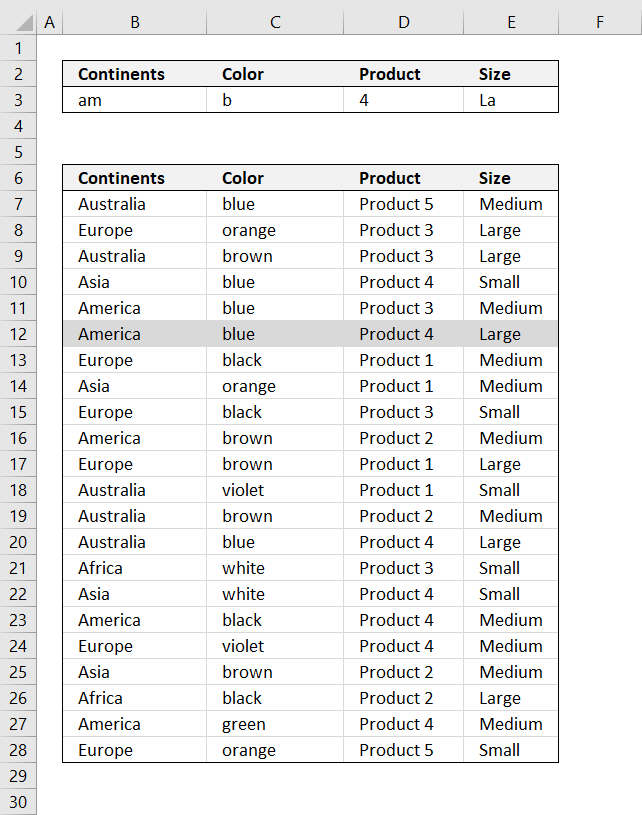
The picture above shows you how to highlight rows containing text strings using conditional formatting.
Example, continents criterion (cell B3) is only searched in column Continents (B7:B28). Color criterion is searched for in column Color, and so on.
Conditional formatting formula:
The formula is not case sensitive. Replace SEARCH function with FIND to make it case sensitive.
How to apply conditional formatting formula
Make sure you adjust cell references to your excel sheet.
- Select cells B6:E27
- Press with left mouse button on "Home" tab
- Press with left mouse button on "Conditional Formatting" button
- Press with left mouse button on "New Rule.."
- Press with left mouse button on "Use a formula to determine which cells to format"
- Type above formula in "Format values where this formula is TRUE" window.
- Press with left mouse button on "Format.." button
- Press with left mouse button on "Fill" tab
- Select a color for highlighted cells.
- Press with left mouse button on "Ok"
- Press with left mouse button on "Ok"
- Press with left mouse button on "Ok"
How the conditional formatting formula works in cell B12
Note, the explanation below is for cell B12. Cell B12 is chosen because it is highlighted by the conditional formatting formula.
Step 1 - Understand relative and absolute cell references
A cell reference may or may not have dollar signs in front of the reference, it indicates the cell reference is fixed meaning it won't change when the cell is copied to other cells.
Example, cell reference $D3 is fixed to column D (absolute cell reference), however, row number 3 changes (relative cell reference) when the cell is copied to another cell.
Step 2 - Search cells to see if criteria are found
The SEARCH function returns the number of the character at which a specific character or text string is found reading left to right (not case-sensitive).
=COUNT(SEARCH($B$3, $B7)+1/($B7<>""))*COUNT(SEARCH($C$3, $C7)+1/($C7<>""))*COUNT(SEARCH($D$3, $D7)+1/($D7<>""))*COUNT(SEARCH($E$3, $E7)+1/($E7<>""))
becomes
=COUNT(SEARCH("am", $B12)+1/($B12<>""))*COUNT(SEARCH("b", $C12)+1/($C12<>""))*COUNT(SEARCH("4", $D12)+1/($D12<>""))*COUNT(SEARCH("LA", $E12)+1/($E12<>""))
becomes
=COUNT(SEARCH("am", "America")+1/("America"<>""))*COUNT(SEARCH("b", "blue")+1/("blue"<>""))*COUNT(SEARCH("4", "Product 4")+1/("Product 4"<>""))*COUNT(SEARCH("LA", "Large")+1/("Large"<>""))
becomes
=COUNT(1+1/("America"<>""))*COUNT(1+1/("blue"<>""))*COUNT(9+1/("Product 4"<>""))*COUNT(1+1/("Large"<>""))
Step 3 - Identify empty criteria and return TRUE or FALSE
The COUNT function counts all numerical values in an argument.
=COUNT(1+1/("America"<>""))*COUNT(1+1/("blue"<>""))*COUNT(9+1/("Product 4"<>""))*COUNT(1+1/("Large"<>""))
becomes
=COUNT(1+1/(TRUE))*COUNT(1+1/(TRUE))*COUNT(9+1/(TRUE))*COUNT(1+1/(TRUE))
becomes
=COUNT(1+1)*COUNT(1+1)*COUNT(9+1)*COUNT(1+1)
becomes
=COUNT(2)*COUNT(2)*COUNT(10)*COUNT(2)
and returns 1 (TRUE). Row 12 is highlighted
8. Highlight lookup values
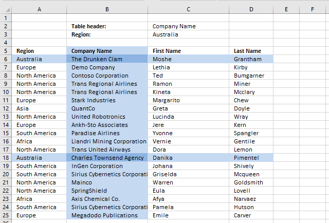
In this article, I will demonstrate how to search a table using conditional formatting. The criteria highlight matching column and rows.
I am also going to explain how to create the highlighting and the conditional formatting formulas behind.

Setting up Conditional Formatting
- Select cell range A5:D25.
- Go to tab "Home".
- Press with left mouse button on the "Conditional formatting" button.
- Press with left mouse button on "New Rule..".
- Press with left mouse button on "Use a formula to determine which cells to format".

- Type conditional formatting formula.
- Press with left mouse button on "Format..." button.
- Select a color.
- Press with left mouse button on OK.
- Press with left mouse button on OK.
Repeat the above steps and create new conditional formatting rules with these formulas and colors:

and

Explaining conditional formatting formulas
It is important to understand how relative and absolute cell references work when it comes to conditional formatting. Remember that cell range A5:D25 was selected before you created the conditional formatting rules, that will be the range the conditional formatting is applied to.
The first conditional formatting formula is:
There are two logical expressions in this formula
- (A$5=$C$2)
- ($A5=$C$3)
They return TRUE if the condition is met or FALSE if not. The asterisk multiplies the boolean values and that will create AND logic between these two logical expressions.
This means that if both expressions return TRUE then the formula returns TRUE or the equivalent numerical value. TRUE is 1 and FALSE is 0 (zero).
Expression 1 Expression 2
TRUE * TRUE = TRUE
FALSE * TRUE = FALSE
TRUE * FALSE = FALSE
FALSE * FALSE = FALSE
The parentheses determine the order of calculation, we want to evaluate the equal signs first and then multiply the expressions.
Step 1 - Highlight cells that have a column header equal to the value in $C$2.
(A$5=$C$2)
The cell reference A$5 changes in each cell in cell range A5:D25 but remember only the column reference changes the row part has a $ indicating it is locked. This makes the formula compare column headers only.
Example, in cell B7, the cell reference changes to:
(B$5=$C$2)
and becomes
"Company Name"="First Name"
and returns FALSE. Column B is not highlighted.
Step 2 - Highlight cells that have a Region value equal to the value in $C$3
($A5=$C$3)
The cell reference $A5 changes in each cell in cell range A5:D25, only the row reference changes.
Example,
In cell B7, the cell reference changes to:
($A7=$C$3)
becomes
"Europe"="Africa"
and returns FALSE.
Step 3 - Check if both criteria are TRUE
=(A$5=$C$2)*($A5=$C$3)
becomes
=FALSE*FALSE
and returns 0. Cell B7 is not highlighted with the selected color.
Recommended links
You can do a lot of interesting stuff with conditional formatting. You can search for cell values containing text strings or highlight records in a list. You can find many more examples in the conditional formatting category.
Recommended reading
Built-in conditional formatting
Data Bars Color scales IconsHighlight cells rule
Highlight cells containing stringHighlight a date occuring
Conditional Formatting Basics
Highlight unique/duplicates
Top bottom rules
Highlight top 10 valuesHighlight top 10 % values
Highlight above average values
Basic CF formulas
Working with Conditional Formatting formulasFind numbers in close proximity to a given number
Highlight empty cells
Highlight text values
Search using CF
Highlight records – multiple criteria [OR logic]Highlight records [AND logic]
Highlight records containing text strings (AND Logic)
Highlight lookup values
Unique distinct
How to highlight unique distinct valuesHighlight unique values and unique distinct values in a cell range
Highlight unique values in a filtered Excel table
Highlight unique distinct records
Duplicates
How to highlight duplicate valuesHighlight duplicates in two columns
Highlight duplicate values in a cell range
Highlight smallest duplicate number
Highlight more than once taken course in any given day
Highlight duplicates with same date, week or month
Highlight duplicate records
Highlight duplicate columns
Highlight duplicates in a filtered Excel Table
Compare
Highlight missing values between to columnsCompare two columns and highlight values in common
Compare two lists of data: Highlight common records
Compare tables: Highlight records not in both tables
How to highlight differences and common values in lists
Compare two columns and highlight differences
Min max
Highlight smallest duplicate numberHow to highlight MAX and MIN value based on month
Highlight closest number
Dates
Advanced Date Highlighting Techniques in ExcelHow to highlight MAX and MIN value based on month
Highlight odd/even months
Highlight overlapping date ranges using conditional formatting
Highlight records based on overlapping date ranges and a condition
Highlight date ranges overlapping selected record [VBA]
How to highlight weekends [Conditional Formatting]
How to highlight dates based on day of week
Highlight current date
Misc
Highlight every other rowDynamic formatting
Advanced Techniques for Conditional Formatting
Highlight cells based on ranges
Highlight opposite numbers
Highlight cells based on coordinates
Excel categories
7 Responses to “Working with Conditional Formatting formulas”
Leave a Reply
How to comment
How to add a formula to your comment
<code>Insert your formula here.</code>
Convert less than and larger than signs
Use html character entities instead of less than and larger than signs.
< becomes < and > becomes >
How to add VBA code to your comment
[vb 1="vbnet" language=","]
Put your VBA code here.
[/vb]
How to add a picture to your comment:
Upload picture to postimage.org or imgur
Paste image link to your comment.
Brilliant! add data validation for the cell C2 and C3 and it makes the job even easier.
Cyril,
Thanks!
Here is the same file with data validation lists in cell C2 and C3:
Search-with-conditional-formatting-data-validation.xlsx
pls tell me, if how can i pick data in particular cell instead of highlighting.
e.g. if i want in value of first name or company name or last name in europe region in cell D3. how to do this
gaurav,
Company name
=INDEX($B$6:$D$25;MATCH("Europe", $A$6:$A$25, 0), 1)
First name
=INDEX($B$6:$D$25;MATCH("Europe", $A$6:$A$25, 0), 2)
Last name
=INDEX($B$6:$D$25;MATCH("Europe", $A$6:$A$25, 0), 3)
How to return multiple values using vlookup
I have two formulas I need to combine - might be a nested if statement but I can't seem to get it to work for me...
The first being:
=If(And(len(F2)>0,E2="Yes"),"Cabling Scheduled","Requested")
The second being:
=If(Today()>J2,"Complete","Scheduled")
What I am looking to do is combine both of these to basically output 3 values. If the date of the cabling is greater than the current date, and if cabling is required, and if there is a cabling completed number, it should show as Complete. Otherwise it should show as Requested or scheduled. Requested would be F2 is blank or E2 is no/pending. Scheduled would be if E2 is Yes, and F2 has anything greater than 0 but the date is less than J2.
Awesome stuff, thank you! You just saved my day.
Bob,
thanks.