Highlight unique values in a filtered Excel table

The image above demonstrates unique values highlighted in a filtered Excel Table. I will in this article show how to apply conditional formatting to an Excel Table.
Table of contents
1. Introduction
Why highlight unique values in a filtered Excel Table?
Excel has a built-in feature that highlights unique values, however, it does not work as intended if the Excel Table is filtered. The highlighting feature considers all values even the filtered-out values which is something you may not want. Section 1 describes how to highlight unique values based on visible filtered values in an Excel Table.
What is Conditional Formatting?
Conditional Formatting in Excel is a feature that applies specific formatting to cells that meet predefined conditions. It allows you to highlight and differentiate data dynamically by changing cell attributes such as fill color, font color, and border styles. When data changes conditional formats automatically update to reflect those changes.
What is an Excel Table?
An Excel table is a named object that manages its contents independently from other worksheet data. It provides features for effective data analysis and management, like:
- Calculated columns. A formula that is automatically populated though all cells in a given column.
- Total row. Calculates a sum.
- Auto-filter and sort options. You can filter the data based on conditions and sort from A to Z or small to large or vice versa.
- Automatic expansion. This means that the Excel Table grows or shrinks when data is added or deleted automatically.
Tables typically contain related data in rows and columns but can consist of a single row or column.
What is a filtered Excel Table?
A filtered Excel table displays only the rows that meet specified criteria while hiding others. Filtering allows you to:
- Work with a subset of data without rearranging or moving it.
- Copy, find, edit, format, chart, and print the filtered data.
- Apply filters to multiple columns, with each filter further reducing the displayed data.
What are unique values?
Unique values in Excel are those that appear only once in a list or range. For example, in the list [A, B, C, A, D], the unique values would be B, C, and D. A has a duplicate and is not unique and not included.
What are unique distinct values?
Unique distinct values in Excel include all different values in a list, comprising both unique values and the first instances of duplicate values. For example, in the list [A, B, C, A, D], the unique distinct values would be A, B, C, and D.
What are unique distinct records/rows?
Unique distinct records or rows in Excel refer to rows that are unique based on values in two or more columns. This concept extends the idea of unique distinct values to multiple dimensions. For example, in a table with columns for Name and Address, unique distinct rows would be those where the combination of Name and Address is unique.
How to put the highlighted values at the top?
Moving the highlighted values to the top is convenient because this minimizes scrolling if you work with a larger table.
- Press with right mouse button on with mouse on the highlighted value. A popup menu appears.
- Hover over "Sort" located on the popup menu. A new popup menu appears.
- Press with left mouse button on with left mouse button on "Put selected cell color on top".
1. Highlight unique values in a filtered Excel table
This section demonstrates a conditional formatting formula that allows you to highlight unique values based on a set of filtered values using an Excel Table.
The image above shows an Excel Table that has a filter applied to column B or Table column header name "Category". A conditional formatting formula highlights unique values in cell range C3:C9.
Items "Pencil" and Eraser" are unique because they exist only once each in the filtered Excel Table, Item "Pen" exists in two different cells and are not highlighted.
Conditional Formatting has some amazing built-in features, for example, it lets you highlight unique values in a list without entering a CF formula. If you don't know how to do this using the built-in tool, follow these instructions:
- Select your list.
- Go to "Home" tab on the ribbon.
- Press with left mouse button on the Conditional formatting button.
- Hover over "Highlight Cells Rules".
- Press with left mouse button on "Duplicate values...".
- Change to "Unique".
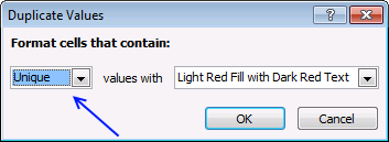
- Press with left mouse button on OK
However, if you then decide to filter the list based on a condition, the CF rule still highlights unique values as if it is not filtered.
The following CF formula highlights unique values in a filtered Excel Table.
The image below shows the filtered Excel table to the left and the same Excel Table to the right, however unfiltered, side by side. The Conditonal Formatting formula is applied to the Table to the left and the built-in tool is applied to the table to the right.

The built-in tool is not able to correctly highlight unique values in a filtered Excel Table, shown below. Item "Pencil" should have been highlighted as well, it is unique in the filtered Excel Table. The Conditional formatting formula, however, is highlighting Item "Pencil" correctly in the Table to the left in the image above.

How to apply a CF formula rule

You probably use a different table name on our worksheet, make sure you change the name accordingly in the CF formula.
- Select the table column or list.
- Go to "Home" tab on the ribbon.
- Press with left mouse button on Conditional formatting button.
- Press with left mouse button on "New rule...".
- Press with left mouse button on "Use a formula to determine which cells to format".
- Paste the above formula in this field.
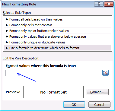
- Press with left mouse button on "Format..." button.
- Go to tab "Fill".
- Pick a background color.
- Press with left mouse button on OK button twice.
Explaining Conditional Formatting formula

I highly recommend the "Evaluate Formula" tool to understand and troubleshoot complicated formulas. It allows you to see calculation steps in greater detail at a pace you can control.
In order to use the "Evaluate Formula" tool you need to copy the CF formula and paste it to a cell next to the Excel Table. Copy the cell and paste to cells below as far as needed.
The image above shows the CF formula in cell E3 and cells below. The cell is highlighted if the CF formula evaluates to the boolean value TRUE.
Select a cell containing the formula you want to understand better, press with left mouse button on the "Formula" tab on the ribbon. Press with left mouse button on the "Evaluate Formula" button, a dialog box appears, see image above.
It shows the formula, the underlined expression is next to be evaluated. The lates evaluated expression is italicized. Press with left mouse button on the "Evaluate" button to see the next calculation step. Press with left mouse button on "Close" button to dismiss the dialog box.
Step 1 - Reference the value in the Excel Table on the same row as the Conditional formatting
Referencing a cell in an Excel Table is different than a regular cell, they are named structured references. First the table name then the column name inside brackets. The @ character tells you that the cell is in the same row as the formula.
Table3[@Item]
The Conditional Formatting formula is applied to cell C3 and Table3[@Item] references the same cell, however, it doesn't have to be the same cell. It can be a different cell but in the same row.
Step 2 - Enable Excel Table references in Conditional Formatting formulas
You can't use structured cell references in a CF formula, however, there is a workaround. Use the INDIRECT function, unfortunately, there is a downside with this approach which is necessary to keep in mind. If you change the name of the Excel Table the structured reference does not change automatically which otherwise would be the case.
INDIRECT("Table3[@Item]")
returns
"Pencil"
Step 3 - Enable arrays in the SUBTOTAL function
The SUBTOTAL function is able to identify if a cell is filtered or not but you can't use an array of values unless you apply this workaround. The OFFSET function is somehow capable of creating an array that you can use in the SUBTOTAL function.
OFFSET(INDIRECT("Table3[Item]"),MATCH(ROW(INDIRECT("Table3[Item]")),ROW(INDIRECT("Table3[Item]")))-1, 0,1))
becomes
OFFSET({"Pencil"; "Pen"; "Marker"; "Eraser"; "Pen"; "Marker"; "Pen"; "Pencil"},MATCH(ROW({"Pencil"; "Pen"; "Marker"; "Eraser"; "Pen"; "Marker"; "Pen"; "Pencil"}")),ROW({"Pencil"; "Pen"; "Marker"; "Eraser"; "Pen"; "Marker"; "Pen"; "Pencil"}))-1, 0,1))
becomes
OFFSET({"Pencil"; "Pen"; "Marker"; "Eraser"; "Pen"; "Marker"; "Pen"; "Pencil"},MATCH({3;4;5;6;7;8;9;10}),{3;4;5;6;7;8;9;10})-1, 0,1))
becomes
OFFSET({"Pencil"; "Pen"; "Marker"; "Eraser"; "Pen"; "Marker"; "Pen"; "Pencil"},{1;2;3;4;5;6;7;8}-1, 0,1))
becomes
OFFSET({"Pencil"; "Pen"; "Marker"; "Eraser"; "Pen"; "Marker"; "Pen"; "Pencil"},{1;2;3;4;5;6;7;8}-1, 0,1))
OFFSET({"Pencil"; "Pen"; "Marker"; "Eraser"; "Pen"; "Marker"; "Pen"; "Pencil"},{0;1;2;3;4;5;6;7}, 0,1))
and returns
{"Pencil";"Pen";"Marker";"Eraser";"Pen";"Marker";"Pen";"Pencil"}
The "Evaluate Formula" tool shows {#VALUE!; #VALUE!; #VALUE!; #VALUE!; #VALUE!; #VALUE!; #VALUE!; #VALUE!} but it still works.
Step 4 - Identify filtered values
SUBTOTAL(3,OFFSET(INDIRECT("Table3[Item]"),MATCH(ROW(INDIRECT("Table3[Item]")),ROW(INDIRECT("Table3[Item]")))-1, 0,1))
becomes
SUBTOTAL(3, {"Pencil";"Pen";"Marker";"Eraser";"Pen";"Marker";"Pen";"Pencil"})
and returns
{1; 1; 0; 1; 0; 0; 1; 0}
1 is visible, 0 (zero is hidden). The order of the values is important, they match the position of the values in column Item.
Step 5 - Replace the array with values
The IF function replaces 1 with the actual value corresponding to the position in the array and returns nothin "" if the value is 0 (zero)
IF(SUBTOTAL(3, OFFSET(INDIRECT("Table3[Item]"), MATCH(ROW(INDIRECT("Table3[Item]")), ROW(INDIRECT("Table3[Item]")))-1, 0, 1)), INDIRECT("Table3[Item]"), "")
becomes
IF({1; 1; 0; 1; 0; 0; 1; 0}, INDIRECT("Table3[Item]"), "")
becomes
IF({1; 1; 0; 1; 0; 0; 1; 0}, {"Pencil";"Pen";"Marker";"Eraser";"Pen";"Marker";"Pen";"Pencil"}, "")
and returns
{"Pencil";"Pen";"";"Eraser";"";"";"Pen";""}
These value are the ones that are visible if you filter column "Category" based on "A".
Step 6 - Count values based on a condition
The COUNTIF function counts the visible values based on a condition which makes it possible to calculate if a value is unique or not.
COUNTIF(INDIRECT("Table3[@Item]"), IF(SUBTOTAL(3, OFFSET(INDIRECT("Table3[Item]"), MATCH(ROW(INDIRECT("Table3[Item]")), ROW(INDIRECT("Table3[Item]")))-1, 0, 1)), INDIRECT("Table3[Item]"), ""))
becomes
COUNTIF(INDIRECT("Table3[@Item]"), {"Pencil";"Pen";"";"Eraser";"";"";"Pen";""})
becomes
COUNTIF("Pencil", {"Pencil";"Pen";"";"Eraser";"";"";"Pen";""})
and returns
{1; 0; 0; 0; 0; 0; 0; 0}
Step 7 - Check if value is unique
The SUM function adds the numbers in the array and returns the total. We know that the value is unique if the total is equal to 1 meaning there is only one instance of that particular value.
SUM(COUNTIF(INDIRECT("Table3[@Item]"), IF(SUBTOTAL(3, OFFSET(INDIRECT("Table3[Item]"), MATCH(ROW(INDIRECT("Table3[Item]")), ROW(INDIRECT("Table3[Item]")))-1, 0, 1)), INDIRECT("Table3[Item]"), "")))=1
becomes
SUM({1; 0; 0; 0; 0; 0; 0; 0})=1
becomes
1=1
and returns True. Cell C3 is highlighted, see image below.
2. Highlight unique distinct values in a cell range
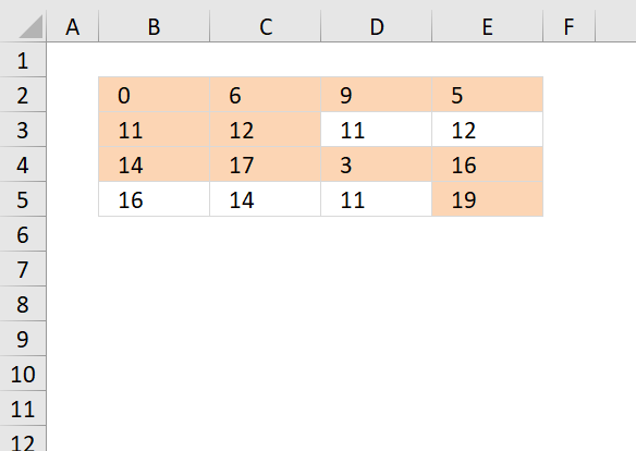
The following formula highlights cells that contain unique distinct values, in other words, all duplicate values except the first instance are not highlighted.
Conditional formatting formula:
How to apply conditional formatting
- Select your range B2:E5.
- Go to "Home" tab on the ribbon.
- Press with left mouse button on "Conditional formatting" button.
- Press with left mouse button on "New Rule.."
- Press with left mouse button on "Use a formula to determine what cells to format"
- Copy the conditional formatting formula above and paste to "Format values where this formula is true:"
- Press with left mouse button on Format button
- Select a formatting.
- Press with left mouse button on OK button.
- Press with left mouse button on OK button.
Explaining CF formula in cell B2
There are two parts in this formula, one part determines if a value is a duplicate in the first column. The second part of the formula determines if a value is a duplicate in the remaining columns.
The reason the formula looks like this is because of the order of how Excel calculates cells.
IF(logical_expression, first_part, second_part)
Step 1 - Check if first column is being evaluated
The COLUMNS function counts columns in a cell reference. $A$1:A1 is an expanding cell reference, it grows because A1 is a relative cell reference that changes between cells.
COLUMNS($A$1:A1)=1
becomes
1=1 and returns TRUE.
Step 2 - Count cells based on a condition
The IF function changes the calculation based on the logical expression in the first argument. The second argument is calculated if the logical expression returns TRUE, the third argument is calculated if the logical expression returns FALSE.
The COUNTIF function makes sure that duplicates are not highlighted, only the first instance of each value. However this works only in the first column, the remaining columns need a different formula in order to do correct calculations.
IF(COLUMNS($A$1:A1)=1,COUNTIF($B$2:B2,B2),COUNTIF($B$2:B2,B2)+COUNTIF(OFFSET($B$2:$E$5,,,4,COLUMNS($A$1:A1)-1),B2))=1
becomes
IF(TRUE,COUNTIF($B$2:B2,B2),...)=1
becomes
IF(TRUE,COUNTIF(0,0),...)=1
becomes
1=1
and returns TRUE. Cell B2 is highlighted.
Step 3 - Calculations in remaining columns
If we move to cell C2 the IF function behaves differently.
IF(COLUMNS($A$1:A1)=1, COUNTIF($B$2:C2, C2), COUNTIF($B$2:C2, C2)+COUNTIF(OFFSET($B$2:$E$5, , , 4, COLUMNS($A$1:B1)-1), C2))=1
becomes
IF(COLUMNS($A$1:B1)=1, COUNTIF($B$2:C2, C2),COUNTIF($B$2:C2, C2)+COUNTIF(OFFSET($B$2:$E$5, , , 4, COLUMNS($A$1:B1)-1), C2))=1
becomes
IF(2=1, COUNTIF($B$2:C2, C2), COUNTIF($B$2:C2, C2)+COUNTIF(OFFSET($B$2:$E$5, , , 4, COLUMNS($A$1:B1)-1), C2))=1
becomes
IF(FALSE, COUNTIF($B$2:C2, C2), COUNTIF($B$2:C2, C2)+COUNTIF(OFFSET($B$2:$E$5, , , 4, COLUMNS($A$1:B1)-1), C2))=1
becomes
IF(FALSE, COUNTIF($B$2:C2, C2), COUNTIF({0,6}, 6)+COUNTIF(OFFSET($B$2:$E$5, , , 4, COLUMNS($A$1:B1)-1), C2))=1
The OFFSET function returns an expanding cell reference that grows as the CF moves from column to column.
IF(FALSE, COUNTIF($B$2:C2, C2), 1+COUNTIF(OFFSET($B$2:$E$5, , , 4, 1), C2))=1
becomes
IF(FALSE, COUNTIF($B$2:C2, C2), 1+COUNTIF($B$2:$B$5, C2))=1
becomes
IF(FALSE, COUNTIF($B$2:C2, C2), 1+COUNTIF({0;11;14;16},6))=1
becomes
IF(FALSE, COUNTIF($B$2:C2, C2), 1+0)=1
becomes
1=1 and returns TRUE. Cell C2 is highlighted.
Get Excel file
highlight unique distinct values in a range.xlsx
3. Highlight unique distinct records
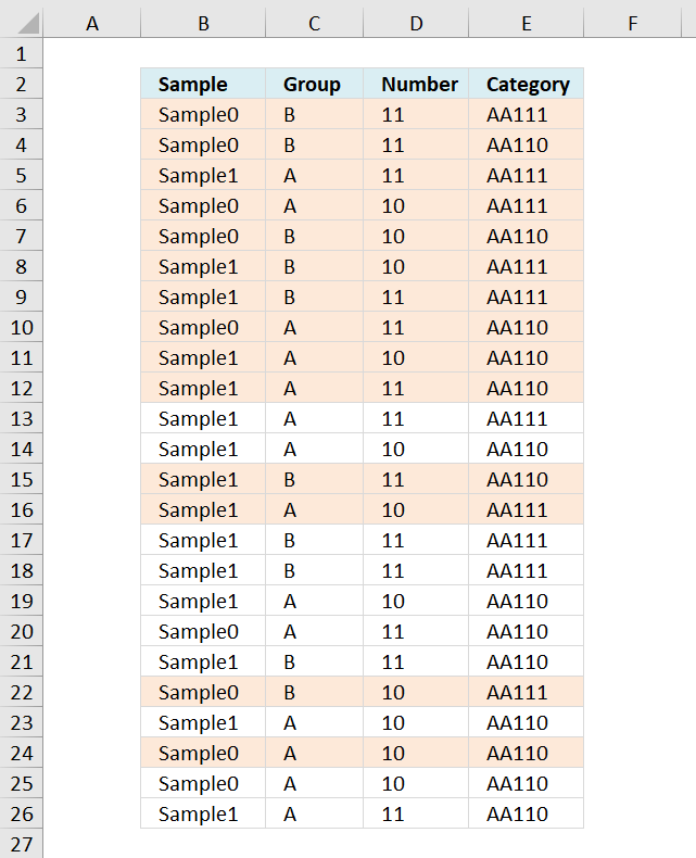
The image above demonstrates a Conditional Formatting formula that highlights unique distinct records. This means that the first instance of each record is highlighted, however, every duplicate is not highlighted.
Example, Row 13 shown in the image above has a duplicate in row 5. Row 5 is the first instance of that particular record and is highlighted but row 13 is a duplicate and is not highlighted.
I have also written an article about how to extract unique distinct records and counting unique distinct records.
Conditional formatting formula:
Explaining condtional formatting formula in cell B3
The COUNTIFS function calculates the number of cells across multiple ranges that equals all given conditions, it has at least one pair of a criteria1 argument and criteria_range1 argument.
COUNTIFS(criteria_range1, criteria1, [criteria_range2, criteria2]…)
In this example we have four columns so 4 pairs are needed to calculate if a record is unique distinct or not.
Step 1 - Absolute and relative cell references
The first argument in the COUNTIFS function is the criteria_range1 and I am using this cell reference: $B$3:$B3
The first part is locked to column B and row 3. $B$3 The second part is only locked to column B, the row number changes as the conditional formatting moves on to the next cell below.
This makes the cell reference grow as the conditional formatting moves to cells below.
The same basic technique is used with the other cell references in the COUNTIFS function.
Step 2 - Count records
COUNTIFS($B$3:$B3, $B3, $C$3:$C3, $C3, $D$3:$D3, $D3, $E$3:$E3, $E3)
becomes
COUNTIFS("Sample0", "Sample0", "B", "B", 11, 11, "AA111", "AA111")
and returns 1.
Step 3 - Check if count is equal to 1
COUNTIFS($B$3:$B3, $B3, $C$3:$C3, $C3, $D$3:$D3, $D3, $E$3:$E3, $E3)=1
becomes
1=1
and returns TRUE. Cell B3 is highlighted.
Recommended reading
Built-in conditional formatting
Data Bars Color scales IconsHighlight cells rule
Highlight cells containing stringHighlight a date occuring
Conditional Formatting Basics
Highlight unique/duplicates
Top bottom rules
Highlight top 10 valuesHighlight top 10 % values
Highlight above average values
Basic CF formulas
Working with Conditional Formatting formulasFind numbers in close proximity to a given number
Highlight empty cells
Highlight text values
Search using CF
Highlight records – multiple criteria [OR logic]Highlight records [AND logic]
Highlight records containing text strings (AND Logic)
Highlight lookup values
Unique distinct
How to highlight unique distinct valuesHighlight unique values and unique distinct values in a cell range
Highlight unique values in a filtered Excel table
Highlight unique distinct records
Duplicates
How to highlight duplicate valuesHighlight duplicates in two columns
Highlight duplicate values in a cell range
Highlight smallest duplicate number
Highlight more than once taken course in any given day
Highlight duplicates with same date, week or month
Highlight duplicate records
Highlight duplicate columns
Highlight duplicates in a filtered Excel Table
Compare
Highlight missing values between to columnsCompare two columns and highlight values in common
Compare two lists of data: Highlight common records
Compare tables: Highlight records not in both tables
How to highlight differences and common values in lists
Compare two columns and highlight differences
Min max
Highlight smallest duplicate numberHow to highlight MAX and MIN value based on month
Highlight closest number
Dates
Advanced Date Highlighting Techniques in ExcelHow to highlight MAX and MIN value based on month
Highlight odd/even months
Highlight overlapping date ranges using conditional formatting
Highlight records based on overlapping date ranges and a condition
Highlight date ranges overlapping selected record [VBA]
How to highlight weekends [Conditional Formatting]
How to highlight dates based on day of week
Highlight current date
Misc
Highlight every other rowDynamic formatting
Advanced Techniques for Conditional Formatting
Highlight cells based on ranges
Highlight opposite numbers
Highlight cells based on coordinates
Excel categories
Leave a Reply
How to comment
How to add a formula to your comment
<code>Insert your formula here.</code>
Convert less than and larger than signs
Use html character entities instead of less than and larger than signs.
< becomes < and > becomes >
How to add VBA code to your comment
[vb 1="vbnet" language=","]
Put your VBA code here.
[/vb]
How to add a picture to your comment:
Upload picture to postimage.org or imgur
Paste image link to your comment.