Conditional Formatting Basics
Table of Contents
- How to add Data Bars to your worksheet
- How to create color scales
- How to insert icons representing cell values
- Highlight cells equal to
- Highlight cells containing string
- Highlight a date occurring...
- Highlight rows/records
- Highlight a row if the date is yesterday
- Highlight a row if the date is today
- Highlight a row if the date is tomorrow
- Highlight a row if the date is in the last 7 days
- Highlight a row if the date is last week
- Highlight a row if the date is in this week
- Highlight a row if the date is in next week
- Highlight a row if the date is in the last month
- Highlight a row if the date is in this month
- Highlight a row if the date is in the next month
- Highlight unique/duplicates
- Highlight top 10 values
- Highlight top 10 % values
- Highlight above average values
1. How to add Data Bars to your worksheet
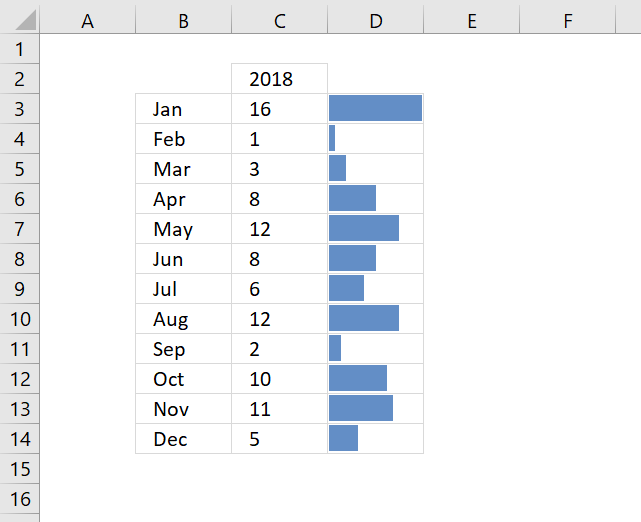
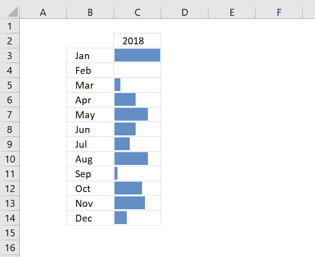
Data bars allows you to insert a data bar into each cell in the selection, the size is based on the cell value. The biggest data bar corresponds to the largest value in selection.
How to build
- Select cells.
- Go to tab "Home" on the ribbon.
- Press with left mouse button on the "Conditional Formatting" button.
- Press with left mouse button on "Data Bars".
- Choose between "Gradient Fill" or "Solid Fill", pick a data bar color to create data bars.
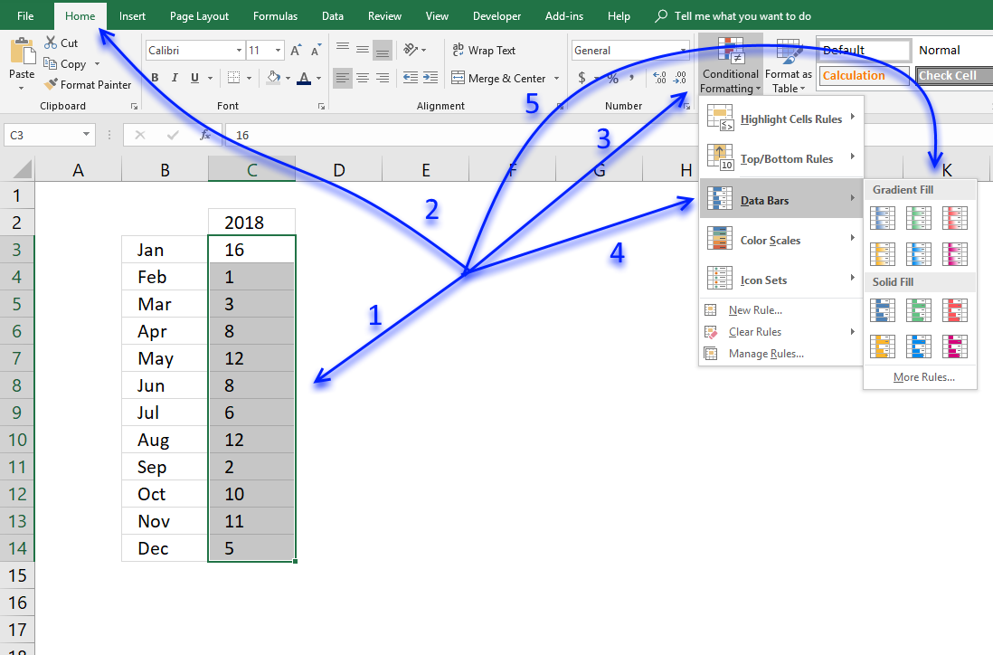
(Press with left mouse button on to expand image)
How to customize data bars
If you want to change data bars settings for an existing cell range follow these steps:
- Select the cell range.
- Go to tab "Home" on the ribbon.
- Press with left mouse button on "Conditional formatting" button.
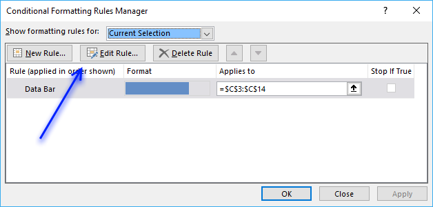
- Press with left mouse button on "Manage Rules..."
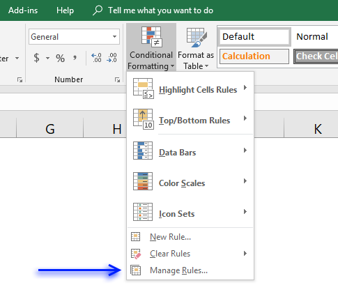
- Press with left mouse button on "Edit Rules..."
To create new data bars and also edit settings before creation then follow these steps:
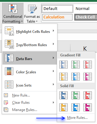
- Select cells.
- Go to tab "Home" on the ribbon.
- Press with left mouse button on the "Conditional Formatting" button.
- Press with left mouse button on "Data Bars".
- Press with left mouse button on "More Rules..."
The data bar settings dialog box appears.
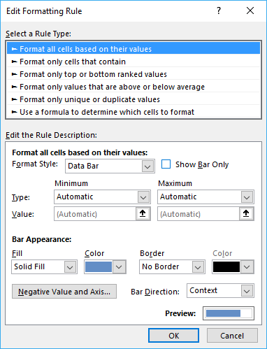
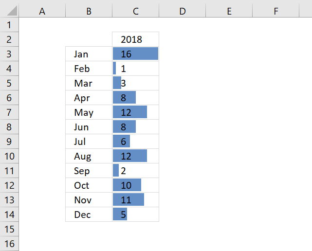
This dialog box lets you format the data bars and how the minimum and maximum values are calculated. You can also hide the values so only the data bars are visible.
I prefer having the values next to the data bars, simply copy the values and paste to the next column then apply the data bars with values hidden.
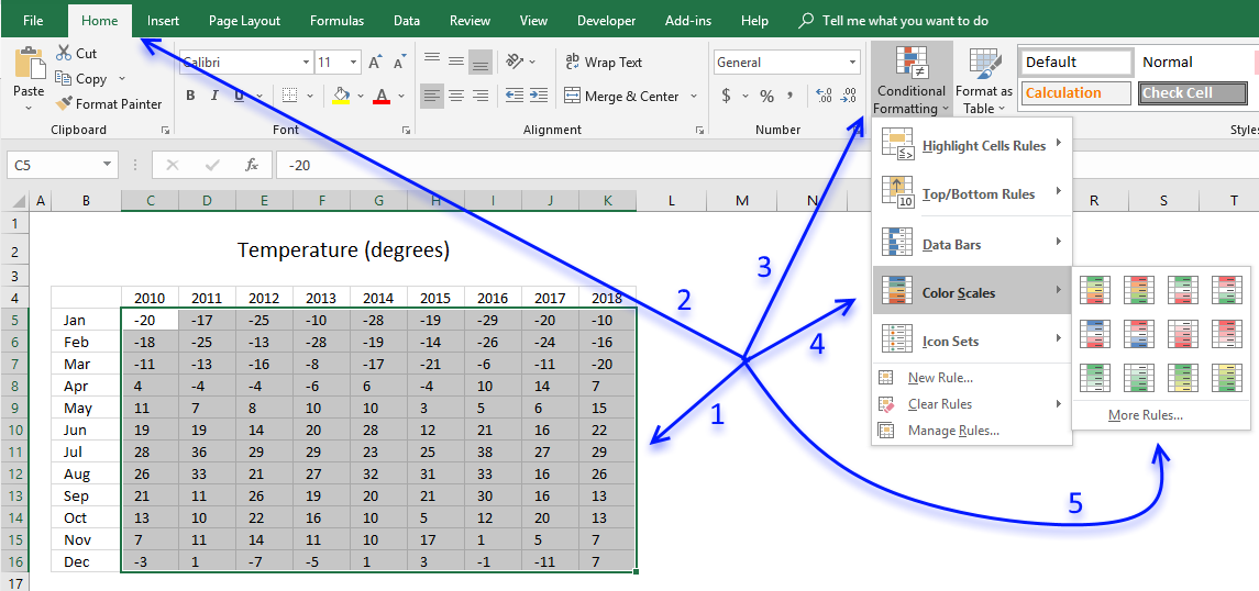
2. How to create color scales
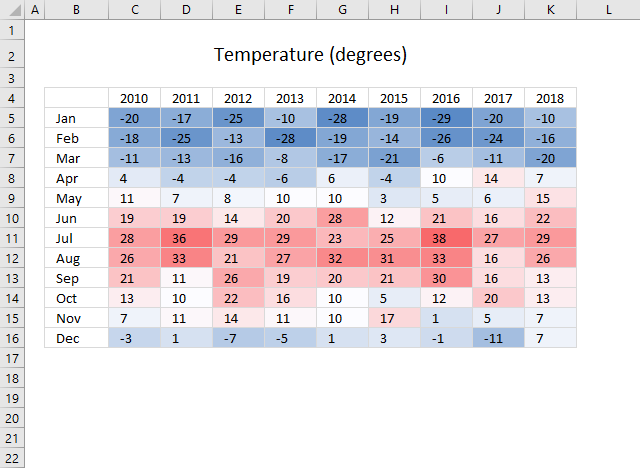
Color scales in conditional formatting applies a color to cells in a cell range based on their values, this lets you easily spot maximum and minimum values as well as trends.
How to build
- Select cell range.
- Go to tab "Home" if you are not already there.
- Press with left mouse button on the "Conditional formatting" button.
- Press with left mouse button on or hover over "Color scales" with the mouse pointer.
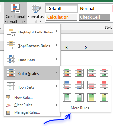
- Pick a predefined color scale or press with left mouse button on "More Rules" to define your own scale and colors.
How to customize Color scales
If you want to change the settings for an existing cell range follow these steps:
- Select the cell range.
- Go to tab "Home" on the ribbon.
- Press with left mouse button on "Conditional formatting" button.
- Press with left mouse button on "Manage Rules..."
- Press with left mouse button on "Edit Rules..."
To create a new color scale and also edit settings before creation then follow these steps:
- Select cells.
- Go to tab "Home" on the ribbon.
- Press with left mouse button on the "Conditional Formatting" button.
- Press with left mouse button on "Color scales".
- Press with left mouse button on "More Rules..."
The settings dialog box appears.
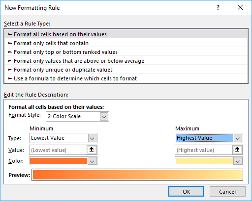
Here you may change the Format style to a 2-Color Scale or 3-Color Scale. The minimum and maximum drop-down lists allow you to change how min and max values are calculated:
- Lowest/Highest
- Number
- Percent
- Formula
- Percentile
3. How to insert icons representing cell values
![]()
Conditional formatting lets you insert icons based on cell values, the idea is to make the data easier to read, for example, spotting small and large values is now quickly done. There are plenty of icon sets to choose from, some have three icons and others have more.
How to build
- Select data.
- Go to tab "Home" on the ribbon if you are not already there.
- Press with left mouse button on the "Conditional formatting" button.
- Press with left mouse button on or hover with mouse pointer on "Icon sets".
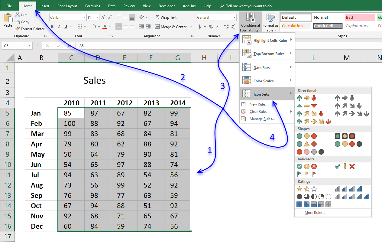
- Pick an icon set. There are four different categories:
- Directional - Arrows
- Shapes - mostly circles
- Indicators
- Ratings - Stars etc.
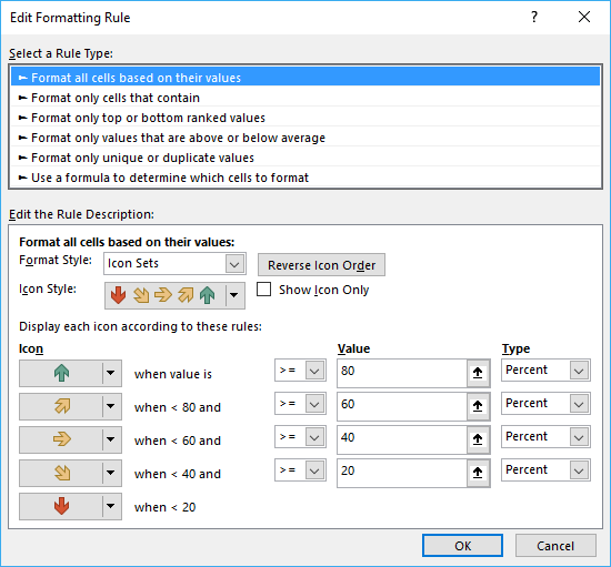
How to customize an icon set
- Select the data.
- Go to tab "Home" on the ribbon.
- Press with left mouse button on the "Conditional formatting" button.
- Press with left mouse button on "Manage Rules..."
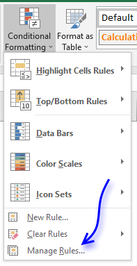
- Press with left mouse button on "Edit" button.
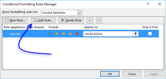
- Here you can change the default settings.
4. Highlight cells equal to
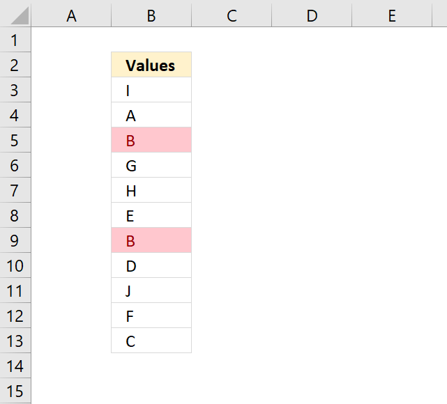
Excel lets you easily highlight values based on a condition you specify, with a built-in formatting or a custom formatting.
How to apply Conditional Formatting to values equal a condition
- Select cell range containing values you want to highlight.
- Go to tab "Home" on the ribbon if you are not already there.
- Press with left mouse button on "Conditional formatting" button.
- Press with mouse on "Highlight Cells Rules".
- Press with left mouse button on "Equal to..."
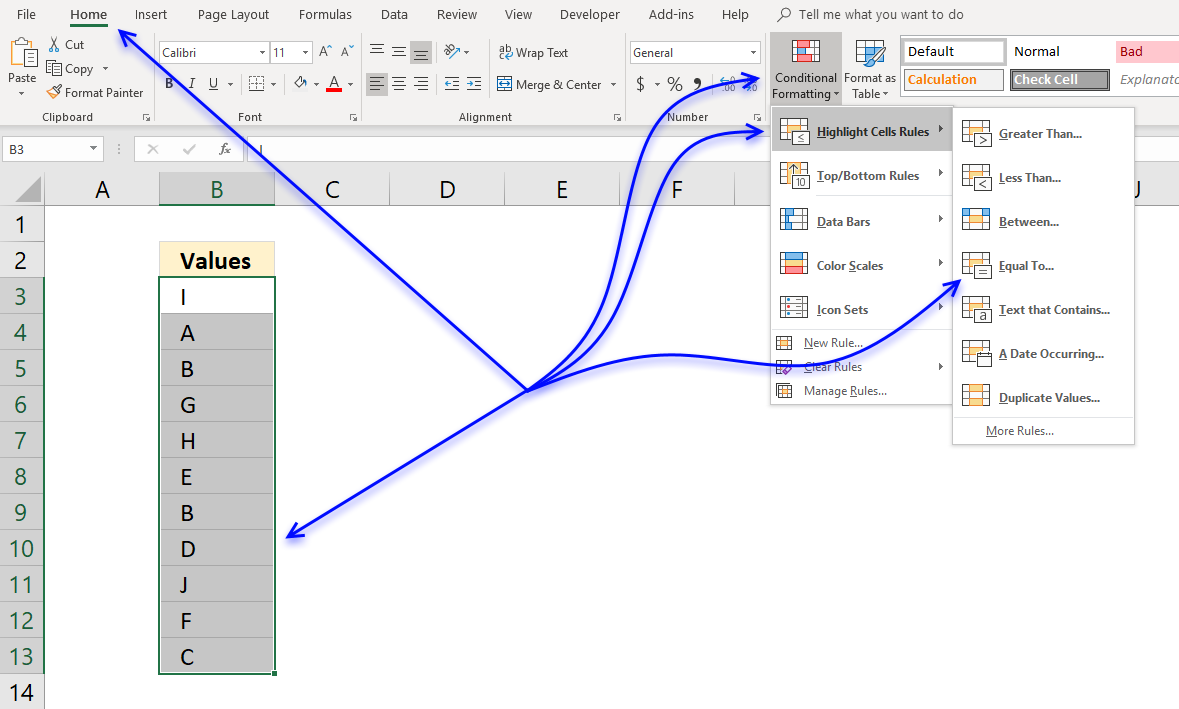
- A dialog box appears that lets you specify the date condition and the formatting.
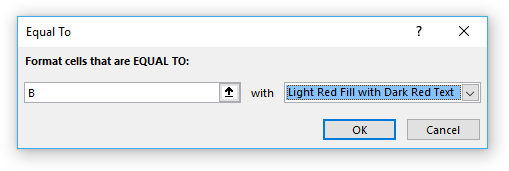
- Pick a prebuilt formatting or use a custom format to create a new one.
- Light red Fill with dark red text
- Yellow fill with dark yellow text
- Green Fill with dark green text
- Light red fill
- Red text
- Red border
- Custom format...
- Press with left mouse button on OK button.
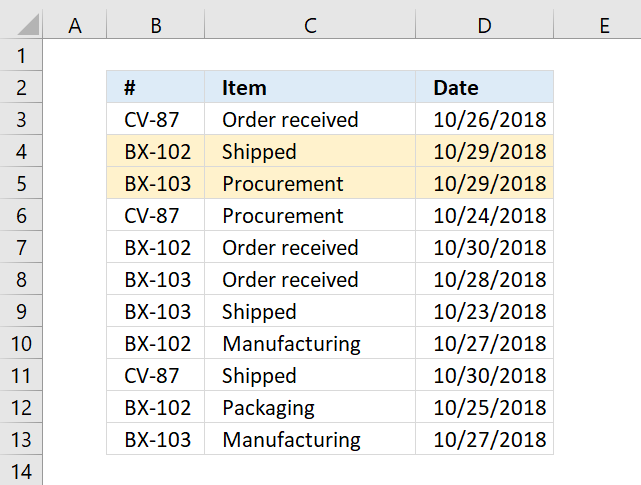
Highlight rows equal to a condition
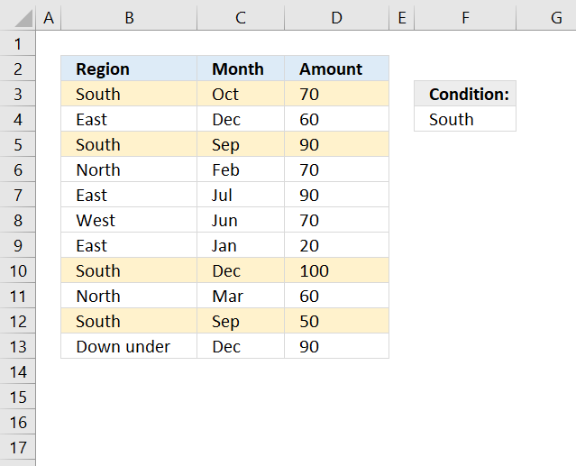
You need to use a formula instead of the prebuilt ones in order to highlight the entire row if a cell in column B meets the condition in cell F4.
- Go to tab "Home" on the ribbon.
- Press with left mouse button on the "Conditional Formatting" button.
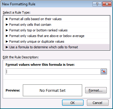
- Press with left mouse button on "New Rule.." to open a dialog box.

- Press with left mouse button on "Use a formula to determine which cells to format".
- Type the formula. (See below).
- Press with left mouse button on "Format..." button and choose a formatting.
- Press with left mouse button on OK button twice.
Conditional formatting formula
Explaining conditional formatting formula
The CF formula changes from cell to cell depending on how you set it up, a cell reference may be absolute or relative.
The dollar sign makes a cell reference locked (absolute), however, a cell reference may also have two dollar signs locking both the column and row. This is the case with $F$4, the condition cell reference never changes.
Cell reference $B3 is only locked to column B, when the CF moves to cell C3 cell ref $B3 is still $B3. This highlights cell C3, see example image above. The next cell is D3 and $B3 is still $B3 highlighting cell D3.
Cell B4 is on the next row and $B3 changes to $B4, cell $B4 is not equal to the condition in cell F4 so this cell is not highlighted and so on.
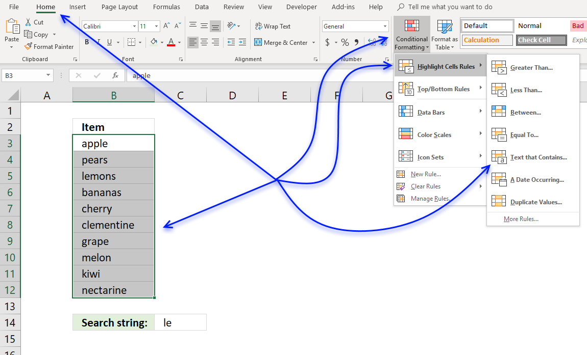
5. Highlight cells containing string
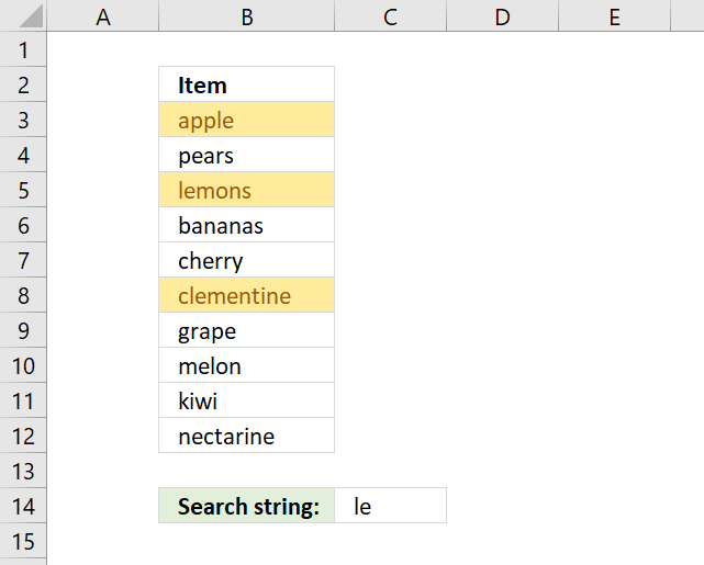
Excel allows you to quickly highlight cells containing a given text string.
How to apply Conditional Formatting
- Select cell range.
- Go to tab "Home" on the ribbon if you are not already there.
- Press with left mouse button on "Conditional formatting" button.
- Press with mouse on "Highlight Cells Rules".
- Press with left mouse button on "Text that Contains..."
- A dialog box appears that lets you specify the text string and the formatting. Press with left mouse button on the arrow to select a cell value that contains the text string to be used, in this case, cell C14.
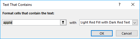
- Pick a formatting or use a custom format.
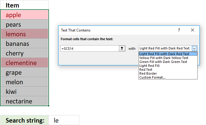
- Press with left mouse button on OK button.
6. Highlight a date occurring...
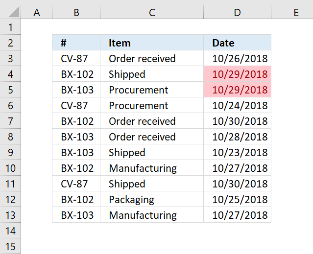
Excel has a built-in feature that allows you to highlight dates if a given condition is met. Section 1 below demonstrates how to create a conditional formatting rule highlighting cells based on date values using the built-in tools. The drop-down list in the dialog box lets you pick from a variety of date conditions:
Yesterday | Today | Tomorrow | In the last 7 days | Last week | This week | Next week | Last month | This month | Next month
Section 2 shows how to create conditional formatting formulas highlighting rows or records in a data set also based on a condition evaluating date values. I will also explain how these conditional formatting formulas work in great detail.
6.1 How to apply Conditional Formatting
- Select cell range containing dates.
- Go to tab "Home" on the ribbon if you are not already there.
- Press with left mouse button on "Conditional formatting" button.
- Press with mouse on "Highlight Cells Rules".
- Press with left mouse button on "A Date Occuring..."
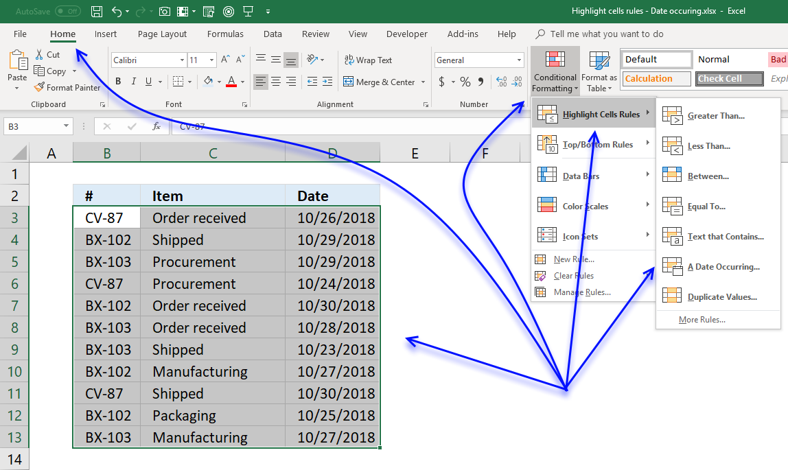
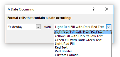
- A dialog box appears that lets you specify the date condition and the formatting.
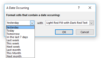
- Pick a prebuilt formatting or use custom format to create a new one.
- Light red Fill with dark red text
- Yellow fill with dark yellow text
- Green Fill with dark green text
- Light red fill
- Red text
- Red border
- Custom format...
- Press with left mouse button on OK button.
7. Highlight rows/records
You need to use a formula instead of the prebuilt ones in order to highlight the entire row if the date meets the condition.
- Go to tab "Home" on the ribbon.
- Press with left mouse button on the "Conditional Formatting" button.
- Press with left mouse button on "New Rule.." to open a dialog box.
- Press with left mouse button on "Use a formula to determine which cells to format".
- Type the formula. (See below which formula to use).
- Press with left mouse button on "Format..." button and choose a formatting.
- Press with left mouse button on OK button twice.
7.1 Highlight a row if the date is yesterday

The following formula highlights all cells on the same row if the date in column D is yesterday:
The $ (dollar sign) makes the cell reference absolute meaning it locks the column thus highlighting all cells on the same row if the date matches the condition.
Read section 2 for instructions on how to insert a conditional formatting formula.
Explaining CF formula in cell D3
Step 1 - Calculate today's date
The TODAY function returns the Excel date (serial number) of the current date.
Function syntax: TODAY()
The TODAY() function is volatile meaning it recalculates more often than regular formulas, this may slow down worksheet calculations.
TODAY()
returns
8/29/2022
Step 2 - Calculate yesterday
The minus sign lets you subtract numbers in an Excel formula.
TODAY()-1
becomes
44802 (8/29/2022)
and returns 44801 (8/28/2022).
Step 3 - Compare yesterday to dates in D3 and cells below
$D3 is both a relative and absolute cell reference, the dollar sign makes D absolute and row number three is a relative cell reference.
This changes the Conditional Formatting formula when a new cell is evaluated, in other words, the row or record is highlighted if the condition is met.
The equal sign lets you compare value to value, the parentheses control the order of operation. We need to calculate yesterday's date before we compare the date numbers.
$D3=(TODAY()-1)
becomes
44802=44801
and returns FALSE. Cell D3 is not highlighted, in fact, no cells on row three are highlighted.
7.2 Highlight a row if the date is today

Conditional formatting formula:
Read section 2 for instructions on how to insert a conditional formatting formula.
Explaining formula
Read section 2.1 Highlight a row if the date is yesterday above for an explanation.
7.3 Highlight a row if the date is tomorrow

Conditional formatting formula:
Read section 2 for instructions on how to insert a conditional formatting formula.
Explaining CF formula in cell D3
Step 1 - Calculate today's date
The today function returns the Excel date (serial number) of the current date.
Function syntax: TODAY()
The TODAY() function is volatile meaning it recalculates more often than regular formulas, this may slow down worksheet calculations.
TODAY()
returns
8/29/2022
Step 2 - Calculate yesterday
The plus sign lets you add numbers in an Excel formula.
TODAY()+1
becomes
44802 (8/29/2022)
and returns 44803 (8/30/2022).
Step 3 - Compare yesterday to dates in D3 and cells below
$D3 is both a relative and absolute cell reference, the dollar sign makes D absolute and row number three is a relative cell reference.
This changes the Conditional Formatting formula when a new cell is evaluated, in other words, the row or record is highlighted if the condition is met.
The equal sign lets you compare value to value, the parentheses control the order of operation. We need to calculate yesterday's date before we compare the date numbers.
$D3=(TODAY()-1)
becomes
44802=44803
and returns FALSE. Cell D3 is not highlighted, in fact, no cells on row three are highlighted.
7.4 Highlight a row if the date is in the last 7 days

Read section 2 for instructions on how to insert a conditional formatting formula.
Explaining CF formula in cell D3
Step 1 - Calculate today's date
The today function returns the Excel date (serial number) of the current date.
Function syntax: TODAY()
The TODAY() function is volatile meaning it recalculates more often than regular formulas, this may slow down worksheet calculations.
TODAY()
returns
44802 (8/29/2022).
Step 2 - Calculate seven days back
TODAY()-7
becomes
44802-7
and returns
44795 (8/22/2022).
Step 3 - Check if the date in cell $D3 is equal or larger than seven days back counting from today
The larger than, smaller than, and the equal sign are logical operators, they return TRUE if the condition is met and FALSE if not.
$D3>=(TODAY()-7)
becomes
44802>=44795
and returns TRUE.
Step 4 - Check if the date in $D3 is smaller or equal to today's date
$D3<=TODAY()
becomes
44802>=44802
and returns TRUE.
Step 5 - Apply AND logic, both conditions must be true
The asterisk character lets you multiply numbers and boolean values in an Excel formula, this applies AND logic to boolean values.
TRUE * TRUE = TRUE
TRUE * FALSE = FALSE
FALSE * FALSE = FALSE
This means that both values must be TRUE to return TRUE (AND logic).
The parentheses control the order of operation, we need to compare values before we multiply.
($D3>=(TODAY()-7))*($D3<=TODAY())
becomes
(TRUE)*(TRUE)
and returns 1. Boolean values are converted to their numerical equivalents. TRUE - 1, FALSE - 0 (zero).
7.5 Highlight a row if the date is in the last week

Change the second argument in WEEKNUM function if the week doesn't begin with Sunday.
Read section 2 for instructions on how to insert a conditional formatting formula.
Explaining CF formula in cell D3
Step 1 - Calculate today's date
The today function returns the Excel date (serial number) of the current date.
Function syntax: TODAY()
The TODAY() function is volatile meaning it recalculates more often than regular formulas, this may slow down worksheet calculations.
TODAY()
returns
44802 (8/29/2022).
Step 2 - Calculate the current week's number
The WEEKNUM function calculates a given date's week number based on a return_type parameter that determines which day the week begins.
Function syntax: WEEKNUM(serial_number,[return_type])
WEEKNUM(TODAY(),1)
becomes
WEEKNUM(44802,1)
and returns 36.
Step 3 - Calculate the last week's number
The minus sign lets you subtract numbers in an Excel formula.
WEEKNUM(TODAY(),1)-1
becomes
36-1
and returns 35.
Step 4 - Check if week's number is equal to last week's number
The larger than, smaller than, and the equal sign are logical operators, they return TRUE if the condition is met and FALSE if not.
WEEKNUM($D3,1)=(WEEKNUM(TODAY(),1)-1)
becomes
36=35
and returns FALSE. Row 3 is not highlighted.
7.6 Highlight a row if the date is in this week

Change the second argument in WEEKNUM function if the week doesn't begin with Sunday.
Read section 2 for instructions on how to insert a conditional formatting formula.
Explaining CF formula in cell D3
Step 1 - Calculate today's date
The today function returns the Excel date (serial number) of the current date.
Function syntax: TODAY()
The TODAY() function is volatile meaning it recalculates more often than regular formulas, this may slow down worksheet calculations.
TODAY()
returns
44802 (8/29/2022).
Step 2 - Calculate the current week's number
The WEEKNUM function calculates a given date's week number based on a return_type parameter that determines which day the week begins.
Function syntax: WEEKNUM(serial_number,[return_type])
WEEKNUM(TODAY(),1)
becomes
WEEKNUM(44802,1)
and returns 36.
Step 3 - Check if week's number is equal to last week's number
The larger than, smaller than, and the equal sign are logical operators, they return TRUE if the condition is met and FALSE if not.
WEEKNUM($D3,1)=(WEEKNUM(TODAY(),1))
becomes
36=36
and returns TRUE. Row 3 is not highlighted.
7.7 Highlight a row if the date is in the next week

Change the second argument in WEEKNUM function if the week doesn't begin with Sunday.
Read section 2 for instructions on how to insert a conditional formatting formula.
Explaining CF formula in cell D3
Step 1 - Calculate today's date
The TODAY function returns the Excel date (serial number) of the current date.
Function syntax: TODAY()
The TODAY() function is volatile meaning it recalculates more often than regular formulas, this may slow down worksheet calculations.
TODAY()
returns
44802 (8/29/2022).
Step 2 - Calculate the current week's number
The WEEKNUM function calculates a given date's week number based on a return_type parameter that determines which day the week begins.
Function syntax: WEEKNUM(serial_number,[return_type])
WEEKNUM(TODAY(),1)
becomes
WEEKNUM(44802,1)
and returns 36.
Step 3 - Calculate the last week's number
The plus sign lets you add numbers in an Excel formula.
WEEKNUM(TODAY(),1)+1
becomes
36-1
and returns 35.
Step 4 - Check if week's number is equal to last week's number
The larger than, smaller than, and the equal sign are logical operators, they return TRUE if the condition is met and FALSE if not.
WEEKNUM($D3,1)=(WEEKNUM(TODAY(),1)-1)
becomes
36=35
and returns FALSE. Row 3 is not highlighted.
7.8 Highlight a row if the date is in the last month

Read section 2 for instructions on how to insert a conditional formatting formula.
Explaining CF formula in cell D3
Step 1 - Calculate today's date
The TODAY function returns the Excel date (serial number) of the current date.
Function syntax: TODAY()
TODAY()
returns
44802 (8/29/2022).
Step 2 - Calculate today's year
The YEAR function converts a date to a number representing the year in the date.
Function syntax: YEAR(serial_number)
YEAR(TODAY())
becomes
YEAR(44802)
and returns 2022.
Step 3 - Calculate today's month number
The MONTH function extracts the month as a number from an Excel date.
Function syntax: MONTH(serial_number)
MONTH(TODAY())
becomes
MONTH(44802)
and returns 8.
Step 4 - Subtract month number by 1
To get last month we need to subtract the month number by 1. The minus character lets you subtract numbers in an Excel formula.
MONTH(TODAY())-1
becomes
8-1
and returns 7.
Step 5 - Concatenate strings
The ampersand character lets you merge strings in an Excel formula.
YEAR(TODAY())&"-"&MONTH(TODAY())-1
becomes
2022&"-"&7
and returns 2022-07
Step 6 - Calculate year and month from date
The TEXT function converts a value to text in a specific number format.
Function syntax: TEXT(value, format_text)
TEXT($D3,"YYYY-M")
becomes
TEXT(44802,"YYYY-M")
and returns
2022-8
Step 7 - Compare strings
The equal sign lets you compare values in an Excel formula, the result is a boolean value TRUE or FALSE.
TEXT($D3,"YYYY-M")=(YEAR(TODAY())&"-"&MONTH(TODAY())-1)
becomes
"2022-8"="2022-7"
and returns FALSE. Cell D3 is not highlighted.
7.9 Highlight a row if the date is in this month

Read section 2 for instructions on how to insert a conditional formatting formula.
Explaining CF formula in cell D3
Step 1 - Calculate today's date
The TODAY function returns the Excel date (serial number) of the current date.
Function syntax: TODAY()
TODAY()
returns
44802 (8/29/2022).
Step 2 - Calculate today's year and month
The TEXT function converts a value to text in a specific number format.
Function syntax: TEXT(value, format_text)
TEXT(TODAY(), "YYYY-M")
becomes
TEXT(44802,"YYYY-M")
and returns
2022-8.
Step 3 - Calculate cell D3's year and month
The TEXT function converts a value to text in a specific number format.
Function syntax: TEXT(value, format_text)
TEXT($D3, "YYYY-M")
becomes
TEXT(44802,"YYYY-M")
and returns
2022-8.
Step 4 - Compare year and month
The equal sign lets you compare values in an Excel formula, the result is a boolean value TRUE or FALSE.
TEXT($D3, "YYYY-M")=TEXT(TODAY(), "YYYY-M")
becomes
"2022-8"="2022-8"
and returns TRUE. Cell D3 is highlighted.
7.10 Highlight a row if the date is in the next month

Read section 2 for instructions on how to insert a conditional formatting formula.
Explaining CF formula in cell D3
Step 1 - Calculate today's date
The TODAY function returns the Excel date (serial number) of the current date.
Function syntax: TODAY()
TODAY()
returns
44802 (8/29/2022).
Step 2 - Calculate today's year
The YEAR function converts a date to a number representing the year in the date.
Function syntax: YEAR(serial_number)
YEAR(TODAY())
becomes
YEAR(44802)
and returns 2022.
Step 3 - Calculate today's month number
The MONTH function extracts the month as a number from an Excel date.
Function syntax: MONTH(serial_number)
MONTH(TODAY())
becomes
MONTH(44802)
and returns 8.
Step 4 - Add 1 to the month number
To get next month we need to add 1 to the month number. The plus character lets you add numbers in an Excel formula.
MONTH(TODAY())+1
becomes
8+1
returns 9.
Step 5 - Concatenate strings
The ampersand character lets you merge strings in an Excel formula.
YEAR(TODAY())&"-"&MONTH(TODAY())+1
becomes
2022&"-"&9
and returns
"2022-9".
Step 6 - Calculate year and month from date
The TEXT function converts a value to text in a specific number format.
Function syntax: TEXT(value, format_text)
TEXT($D3,"YYYY-M")
becomes
TEXT(44802,"YYYY-M")
and returns
"2022-8".
Step 7 - Compare strings
TEXT($D3,"YYYY-M")=(YEAR(TODAY())&"-"&MONTH(TODAY())+1)
becomes
"2022-8"="2022-9"
and returns FALSE.
8. Highlight unique/duplicates
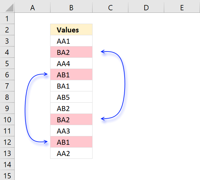
Excel has a few built-in conditional formatting features, one of them highlights values that have at least one duplicate. The other one highlights unique values meaning there is only one instance of the value in the range.
How to apply conditional formatting
- Select the cell range containing the values.
- Go to tab "Home" on the ribbon if you are not already there.
- Press with left mouse button on "Conditional formatting" button.
- Press with mouse on "Highlight Cells Rules".
- Press with left mouse button on "Duplicate values..."
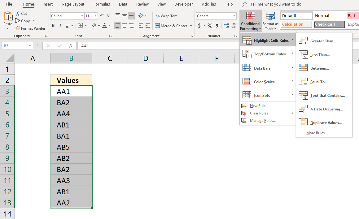
- A dialog box shows up, here you can choose from duplicate or unique .
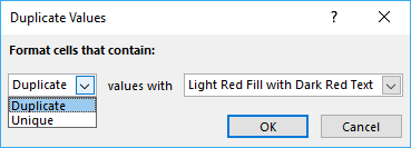
- Choose a formatting you want to apply.
- Light red Fill with dark red text
- Yellow fill with dark yellow text
- Green Fill with dark green text
- Light red fill
- Red text
- Red border
- Custom format...
- If you pick "Custom Format..." the following dialog box appears.
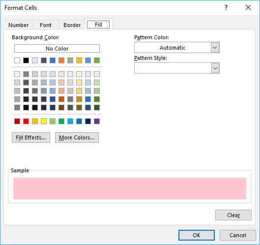
- Press with left mouse button on OK button.
- Press with left mouse button on OK button.
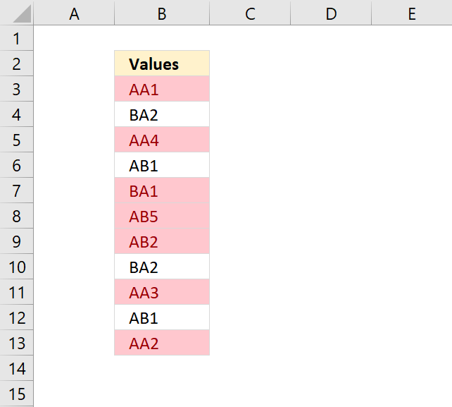
The following image shows unique values highlighted.
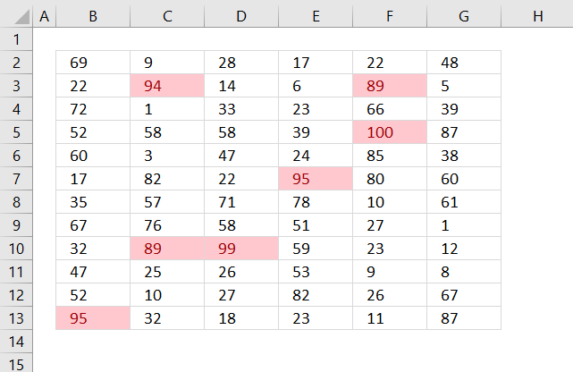
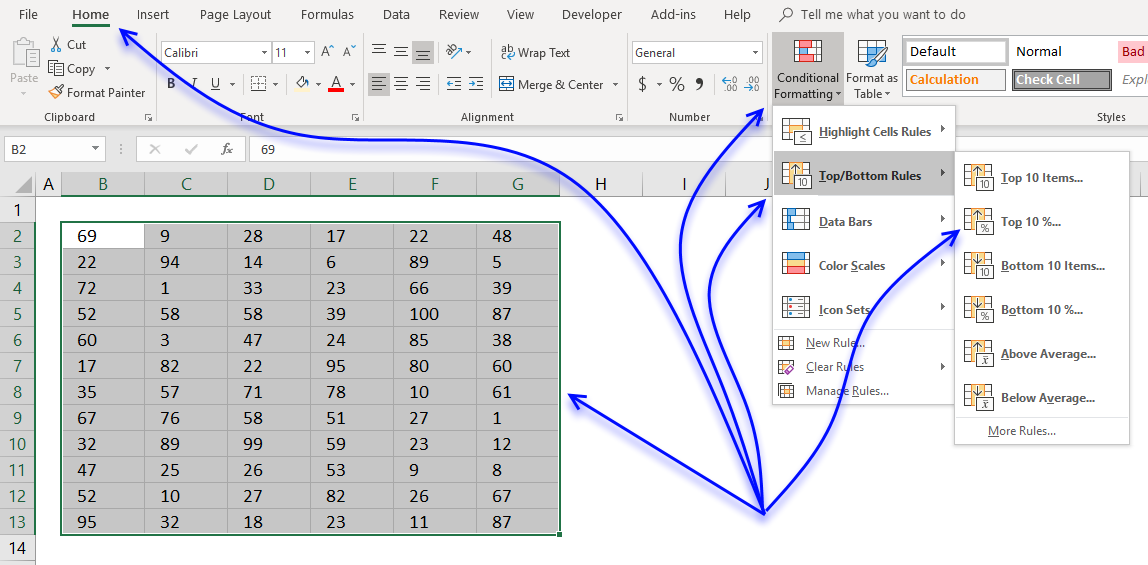
9. Highlight top 10 values
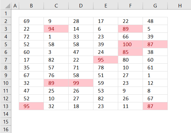
The image above shows top 10 values using conditional formatting applied to cell range B2:G13.
How to format
- Select cell range.
- Go to tab "Home" on the ribbon if you are not already there.
- Press with mouse on "Conditional Formatting" button.
- Press with mouse on "Top/Bottom Rules".
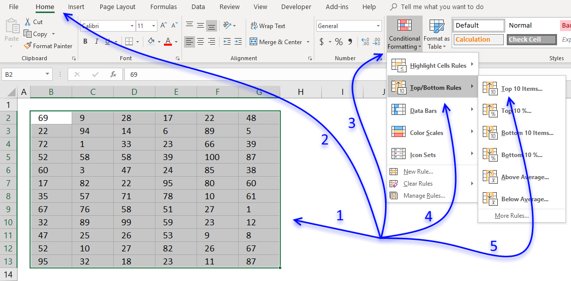
- Press with mouse on "Top 10 Items..."
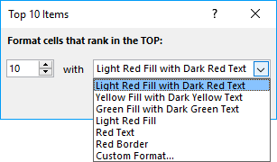
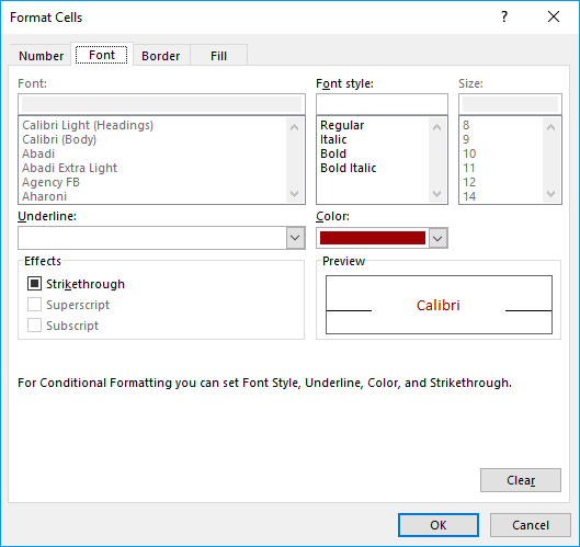
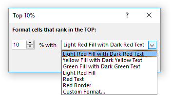
- A dialog box appears see image above, choose how many top items you want to highlight, the default value is 10. The drop-down list contains preconfigured formattings. "Custom Format.." opens another dialog box with more detailed settings.
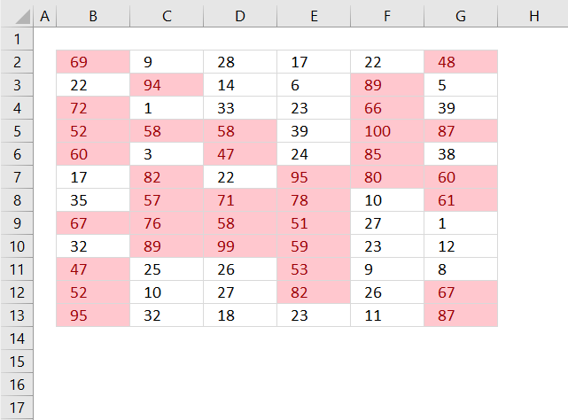
10. Highlight top 10 % values
The image above shows top 10% values using conditional formatting applied to cell range B2:G13. Cell range B2:G13 contains 72 numbers, 10% of 72 is roughly 7. These seven values are then highlighted.
How to format
- Select cell range.
- Go to tab "Home" on the ribbon if you are not already there.
- Press with mouse on "Conditional Formatting" button.
- Press with mouse on "Top/Bottom Rules".
- Press with mouse on "Top 10 %..."
- A dialog box appears see image above, choose how many top items you want to highlight, the default value is 10.
The drop-down list contains preconfigured formattings. "Custom Format.." opens another dialog box with more detailed settings, see image below.
11. Highlight above average values
The image above shows values above average using conditional formatting applied to cell range B2:G13. Cell range B2:G13 contains 72 numbers, the average is approximately 45.39. Values equal to 46 or above are highlighted.
How to format
- Select cell range.
- Go to tab "Home" on the ribbon if you are not already there.
- Press with mouse on "Conditional Formatting" button.
- Press with mouse on "Top/Bottom Rules".
- Press with mouse on "Above Average".
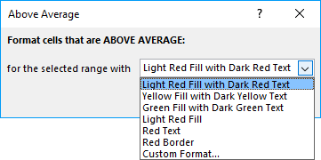
- A dialog box appears, see image above. The drop-down list contains preconfigured formattings. "Custom Format.." opens another dialog box with more detailed settings.
Recommended reading
Built-in conditional formatting
Data Bars Color scales IconsHighlight cells rule
Highlight cells containing stringHighlight a date occuring
Conditional Formatting Basics
Highlight unique/duplicates
Top bottom rules
Highlight top 10 valuesHighlight top 10 % values
Highlight above average values
Basic CF formulas
Working with Conditional Formatting formulasFind numbers in close proximity to a given number
Highlight empty cells
Highlight text values
Search using CF
Highlight records – multiple criteria [OR logic]Highlight records [AND logic]
Highlight records containing text strings (AND Logic)
Highlight lookup values
Unique distinct
How to highlight unique distinct valuesHighlight unique values and unique distinct values in a cell range
Highlight unique values in a filtered Excel table
Highlight unique distinct records
Duplicates
How to highlight duplicate valuesHighlight duplicates in two columns
Highlight duplicate values in a cell range
Highlight smallest duplicate number
Highlight more than once taken course in any given day
Highlight duplicates with same date, week or month
Highlight duplicate records
Highlight duplicate columns
Highlight duplicates in a filtered Excel Table
Compare
Highlight missing values between to columnsCompare two columns and highlight values in common
Compare two lists of data: Highlight common records
Compare tables: Highlight records not in both tables
How to highlight differences and common values in lists
Compare two columns and highlight differences
Min max
Highlight smallest duplicate numberHow to highlight MAX and MIN value based on month
Highlight closest number
Dates
Advanced Date Highlighting Techniques in ExcelHow to highlight MAX and MIN value based on month
Highlight odd/even months
Highlight overlapping date ranges using conditional formatting
Highlight records based on overlapping date ranges and a condition
Highlight date ranges overlapping selected record [VBA]
How to highlight weekends [Conditional Formatting]
How to highlight dates based on day of week
Highlight current date
Misc
Highlight every other rowDynamic formatting
Advanced Techniques for Conditional Formatting
Highlight cells based on ranges
Highlight opposite numbers
Highlight cells based on coordinates
Excel categories
Leave a Reply
How to comment
How to add a formula to your comment
<code>Insert your formula here.</code>
Convert less than and larger than signs
Use html character entities instead of less than and larger than signs.
< becomes < and > becomes >
How to add VBA code to your comment
[vb 1="vbnet" language=","]
Put your VBA code here.
[/vb]
How to add a picture to your comment:
Upload picture to postimage.org or imgur
Paste image link to your comment.