Identify rows of overlapping records
This article demonstrates a formula that points out row numbers of records that overlap the current record based on a start and end date.
What's on this webpage
1. Identify rows of overlapping records - Excel 365

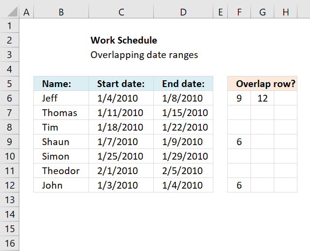
The formula in cell F6 checks whether the date range specified on row 6 overlaps any of the remaining date ranges in cell range F6:D12 and then returns the corresponding row numbers. It always returns the current row number as a result of the date range always overlapping itself.
Excel 365 dynamic formula in cell F6:
1.1 Explaining formula
Step 1 - Calculate row numbers based on a cell reference
The ROW function calculates the row number of a cell reference.
Function syntax: ROW(reference)
ROW($B$6:$B$12) returns {6;7;... ;12}
Step 2 - Check if start date is smaller than or equal to all end dates
The less than and equal signs are logical operators that let you check if a number is smaller or equal to another number.
$C6<=$D$6:$D$12
returns {TRUE; TRUE; ... ; TRUE}.
Step 3 - Check if end date is larger than or equal to all start dates
The larger than and equal signs are logical operators that let you check if a number is smaller or equal to another number.
$D6>=$C$6:$C$12 returns {TRUE; FALSE; ... ; TRUE}.
Step 4 - Multiply arrays (AND logic)
The parentheses let you control the order of operation, we need to evaluate the logical operators before we multiply the arrays.
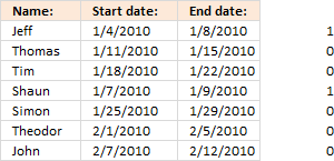
($C6<=$D$6:$D$12)*($D6>=$C$6:$C$12) returns {1;0;0;1;0;0;1}.
Boolean values are converted to their numerical equivalents: 1 - TRUE , 0 (zero) - FALSE.
Step 5 - Filter row numbers based on an array containing boolean values
The FILTER function extracts values/rows based on a condition or criteria.
Function syntax: FILTER(array, include, [if_empty])
FILTER(ROW($B$6:$B$12), ($C6<=$D$6:$D$12)*($D6>=$C$6:$C$12)) returns {6; 9; 12}.
Step 6 - Rearrange vertical values horizontally
The TRANSPOSE function converts a vertical range to a horizontal range, or vice versa.
Function syntax: TRANSPOSE(array)
TRANSPOSE(FILTER(ROW($B$6:$B$12), ($C6<=$D$6:$D$12)*($D6>=$C$6:$C$12)))
2. Identify rows of overlapping records - earlier versions
Hi Oscar,Great website! Keep up the good work.I have a question as to how to expand this to the next step. Per your initial example we can see that Jeff in Row 1 and Shaun in Row 4 overlap their work schedule. I would like to know if there were a way, say for instance in Range E6:E12, to display Jeff’s Row number next to Shaun’s name and visa – versa. I can see how this will easily display what record numbers overlap when there is only one overlap in the range. Can we differentiate the records when there are two overlaps? Let’s say Theodor in Row 6 also has an overlap with Thomas in Row 2.Now the data becomes confusing because we have to determine, from the 4 grayed rows, who overlaps with whom.Can a formula return the Row value of the “matching” overlap record?
In Jeff’s E6 cell it would indicate “Row 4” as to the matching record, and the reverse for Shaun. Shaun’s E9 cell would indicate “Row 1” as the matching record.
And at the same time Theodor’s E11 cell would reflect “Row 2” for Thomas’s record and Thomas’ E7 cell would show “Row 6” for Theodor.I haven’t even touched on the tougher one, such as what happens when John in Row 7 has an end date of 2010-01-07, thus overlapping with both Jeff and Shaun!One step at a time. :)Thanks
The array formula in cell F6 returns the rows of overlapping date ranges for the current record. The record on row 6 overlaps with both records on rows 9 and 12.
Records on row 9 and 12 show they overlap with the record on row 6, this makes it much easier to spot overlapping records.
Formula in cell F6:
How to enter an array formula

You need to enter the formula in cell F6 as an array formula if you have an older Excel version than Excel 365 subscription.
- Copy above array formula (Ctrl + c).
- Double press with left mouse button on cell F6.
- Paste above array formula (Ctrl + v).
- Press and hold CTRL + SHIFT simultaneously.
- Press Enter once.
- Release all keys on keyboard.
The formula now has a beginning and ending curly bracket, like this: {=array_formula}
How to copy array formula

- Select cell F6.
- Press and hold left mouse button on the green dot located at the bottom right corner of the selected cell.
- Drag with the mouse as far as needed to the right.
- Press and hold left mouse button on the green dot located at the bottom right corner of the selected cell range.
- Drag with the mouse downwards as far as needed.
The formula contains relative cell references, they change when the cell is copied. You need to copy cells to get this to work.
Concatenated row numbers

If you rather have row numbers concatenated in a single cell use the following formula.
The TEXTJOIN function is available for Excel 365 subscribers, there is also User Defined Function (UDF) on the same webpage if you own an earlier version of Excel.
Explaining formula in cell F6

I recommend using the "Evaluate Formula" tool located on the Formula tab on the ribbon. Press with left mouse button on the "Evaluate Formula" button, a dialog box appears, see image above.
Press with left mouse button on the Evaluate button to see next calculation step.
Step 1 - Identify overlapping date ranges
The logical operators <> and = allow you to compare dates and find overlapping date ranges.
($B6<=$C$6:$C$12)*($C6>=$B$6:$B$12)
becomes
{1;0;0;1;0;0;1}

If you multiply boolean values you get this in Excel:
- TRUE * TRUE = 1
- TRUE * FALSE = 0
- FALSE *FALSE = 0
This is AND logic and the asterisk allows you to multiply arrays row-wise.

If you use the AND function it will apply AND logic to all values and return a single value, that is the reason we can't use it here.
We want it to return an array so we can easily identify the overlapping date ranges.
The array has the same number of values as there are date ranges, the position in the array corresponds to the position in the list of records.
Step 2 - Create an array containing row numbers except for the current row number
To be able to return the correct row numbers we must create an array that is equally large as the previous array.
We don't want to return the date range for the current record so we need to figure out a way to remove the current row number from the array.
IF(ROW($C$6:$C$12)=ROW(), "", ROW($C$6:$C$12)), "")
becomes
IF({6;7;8;9;10;11;12}=6, "", {6;7;8;9;10;11;12}, "") and returns {"";7;8;9;10;11;12}

Step 3 - If current date range overlaps another date range then return row number
The logical expressions we built in step 1 is now used in an IF function to extract the correct row numbers of date ranges that overlap.
IF(($B6<=$C$6:$C$12)*($C6>=$B$6:$B$12), IF(ROW($B$6:$B$12)=ROW(), "", ROW($B$6:$B$12)), "")
becomes IF({1;0;0;1;0;0;1}, {"";7;8;9;10;11;12}, "") returns {"";"";"";9;"";"";12}

Step 4 - Find the k-th smallest row number
The last step is to extract the smallest number based on where in worksheet the formula is calculated.
SMALL(IF(($B6<=$C$6:$C$12)*($C6>=$B$6:$B$12), IF(ROW($B$6:$B$12)=ROW(), "", ROW($B$6:$B$12)), ""),COLUMN(A1))
The COLUMN function calculates the column number based on a cell reference. The cell reference A1 is relative meaning it changes when the cell is copied to cells to the right.
SMALL({"";"";"";9;"";"";12}, COLUMN(A1)) returns 12 in cell G6.
Recommended articles
How to find overlapping date/time ranges in Excel?
Check if two ranges of dates overlap (Excel Formulas)
3. Identify overlapping date ranges
This section demonstrates formulas that show if a date range is overlapping another date range. The second section shows how to identify overlapping date ranges based on a condition.
Table of Contents
- Identify overlapping date ranges
- Identify overlapping date ranges based on a condition
3.1. Identify overlapping date ranges
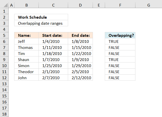
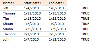
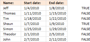
The formula in cell F6 returns TRUE if the date range on the same row overlaps another date range in cell range C6:D12.
Formula in cell F6:
Copy cell E6 and paste it down as far as needed.
If there are multiple overlapping date range it can be quite hard to identify which date range overlaps, I made an article that assists you in finding overlapping date ranges.
There is also a formula for counting overlapping days: Counting overlapping days
Here is a picture of the date ranges. Jeff's and Shaun's date ranges overlap.
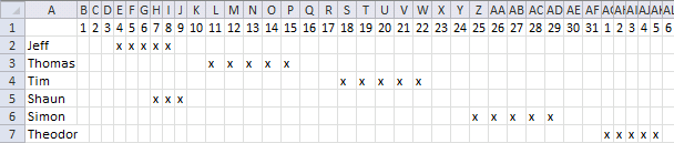
If you are interested in a formula that creates a schedule based on date ranges, like the one above, read the following article: Visualize date ranges in a calendar
Explaining formula in cell F6
I am using date values in this worksheet and Excel handles dates as numbers if you don't know that. For example, 1/1/1900 is 1. 1/1/2018 is 43101.
You can verify this by typing 1/1/1900 in a cell and then press Enter. Select the cell containing the date and press and hold CTRL, then press 1. This opens the "Format Cell" dialog box, here you can change the
Step 1 - Check if start date is less than or equal to end dates
The less than and equal sign allows you to build a logical expression that returns a boolean value.
A boolean value is either TRUE or FALSE. In this case, the expression returns an array of value since we are comparing one date value with multiple date values.
 C6<=$D$6:$D$12
returns
{TRUE; ... ; TRUE}. See the image to the right.
Note that C6 is a relative cell reference that changes when the formula is copied to the cells below. (Actually you copy the cell and paste to the cells below.)
$D$6:$D$12 is an absolute cell reference meaning it won't change when you copy the cell and paste to cells below. Read more: How to use absolute and relative references
Step 2 - Check if end date is larger than or equal to start dates
The next logical expression is somewhat similar to the first one except that now we compare if the end date is larger or equal to the start dates.
 D6>=$C$6:$C$12
returns an array displayed in the image to the right.
Step 3 - Multiply arrays
This step multiplies the arrays, this means AND logic between values on the same row.
(C6<=$D$6:$D$12)*(D6>=$C$6:$C$12)
returns an array displayed in the image to the right.
The parentheses are necessary so the logical operators are performed first and then arrays being multiplied.
 Multiplying arrays containing boolean values converts them into their numerical counterparts. TRUE = 1 and FALSE = 0.
TRUE * TRUE = 1
TRUE * FALSE = 0
FALSE * FALSE = 0
This is called AND logic. The image shows that the first date range and the fourth date range overlap the first date range.
Step 4 - Sum values in array
SUMPRODUCT((C6<=$D$6:$D$12)*(D6>=$C$6:$C$12))
becomes
SUMPRODUCT({1;0;0;1;0;0;0})
and returns 2.
This means that there are two date ranges overlapping. The one we are comparing with, of course, is overlapping and another one on row 4.
Step 5 - Check if sum is larger than 1
SUMPRODUCT((C6<=$D$6:$D$12)*(D6>=$C$6:$C$12))>1
becomes
2>1 returns TRUE in cell F6.
Final notes
If you are only comparing one date range with another you can simply use the MEDIAN function.
3.2. Find overlapping date ranges with criterion
Brett asks:
Hey Oscar,
I tried this and I can't get accurate results with the data set I'm working with.
As an example, how would the formula work if I wanted to find the overlap between the start 2/end 2 dates versus start 1/end 1 dates?
Title - Start 1 End 1 Start 2 End 2 Overlap?
Titans 6/1/14 5/31/15 6/1/14 6/30/14
Titans 6/1/16 5/31/17 8/1/14 8/31/14
Titans 6/1/18 5/31/19 6/1/17 5/31/18
Titans 7/1/21 6/30/23 6/1/19 2/29/20
In the above example, in the "overlap" cell, it should say "yes" for row 1 and row 2, and "no" for row 3 and row 4.
Thanks so much for the help!
Answer:

This example demonstrates a formula that identifies overlapping date range based on two date ranges and a condition specified in column A. The first date range specified in cells B2:C2 is compared to date ranges in columns D and E.
The second date range specified in cells D2:E2 is compared to date ranges in columns B and C.
Formula in cell F2:
Explaining formula
Step 1 - Check if start date in cell B2 is smaller than or equal to end dates in cells $E$2:$E$5
The smaller than, larger than, and the equal characters are logical operators that allow you to compare Excel dates. Excel dates are regular numbers, 1 is 1/1/1900 and 2 represents 1/2/1900, and so on.
The result is a boolean value TRUE or FALSE based on if the condition is met or not.
returns {TRUE; TRUE; TRUE; TRUE}.
Step 2 - Check if end date in cell C2 is larger than or equal to start dates in cells $D$2:$D$5
C2>=$D$2:$D$5
returns {TRUE; TRUE; FALSE; FALSE}
Step 3 - Multiply arrays (AND logic)
The asterisk character lets you multiply numbers in an Excel formula, this works also fine with arrays.
In other words, both values must be TRUE to return TRUE. The equivalent to TRUE is 1 and FALSE is 0 (zero), this is the result after multiplying Boolean values.
The parentheses are needed to control the order of operation, we need to perform the comparisons before we multiply the arrays.
(B2<=$E$2:$E$5)* (C2>=$D$2:$D$5)
returns {1; 1; 0; 0}.
Step 4 - Check if the start date in cell D2 is smaller than or equal to end dates in cells $C$2:$C$5
D2<=$C$2:$C$5
returns {TRUE; TRUE; TRUE; TRUE}.
Step 5 - Check if end date in cell E2 is larger than or equal to start dates in cells $B$2:$B$5
E2>=$B$2:$B$5
returns {TRUE; FALSE; FALSE; FALSE}.
Step 6 - Multiply arrays (AND logic)
(D2<=$C$2:$C$5)* (E2>=$B$2:$B$5)
returns {1;0;0;0}.
Step 7 - Add arrays (OR logic)
The plus sign lets you add numbers in an Excel formula, it also lets you apply OR logic to boolean values.
The result after adding boolean values is their numerical equivalents, TRUE is 1 and FALSE is 0 (zero).
(B2<=$E$2:$E$5)* (C2>=$D$2:$D$5)+ (D2<=$C$2:$C$5)* (E2>=$B$2:$B$5)
becomes
{1; 1; 0; 0} + {1; 0; 0; 0}
and returns {2; 1; 0; 0}.
Step 8 - Check if condition in cell A2 matches cells $A$2:$A$5
A2=$A$2:$A$5
returns {TRUE; TRUE; TRUE; TRUE}.
Step 9 - Multiply arrays (AND logic)
(A2=$A$2:$A$5)* ((B2<=$E$2:$E$5)* (C2>=$D$2:$D$5)+ (D2<=$C$2:$C$5)* (E2>=$B$2:$B$5))
returns {2; 1; 0; 0}.
Step 10 - Add values
The SUMPRODUCT function calculates the product of corresponding values and then returns the sum of each multiplication.
Function syntax: SUMPRODUCT(array1, [array2], ...)
SUMPRODUCT((A2=$A$2:$A$5)* ((B2<=$E$2:$E$5)* (C2>=$D$2:$D$5)+ (D2<=$C$2:$C$5)* (E2>=$B$2:$B$5)))
returns 3.
Step 11 - Check if number is larger than 0 (zero)
SUMPRODUCT((A2=$A$2:$A$5)* ((B2<=$E$2:$E$5)* (C2>=$D$2:$D$5)+ (D2<=$C$2:$C$5)* (E2>=$B$2:$B$5)))>0
3>0
returns TRUE.
4. Filter overlapping date ranges

This blog section describes how to extract coinciding date ranges using array formulas, the image above shows random date ranges in cell range B3:C25.
Table of Contents
- Filter overlapping date ranges
- Filter overlapping date ranges - Excel 365
4.1. Filter overlapping date ranges
Overlapping date ranges
Array formula in cell E4:
To enter an array formula, type the formula in a cell then press and hold CTRL + SHIFT simultaneously, now press Enter once. Release all keys.
The formula bar now shows the formula with a beginning and ending curly bracket telling you that you entered the formula successfully. Don't enter the curly brackets yourself.
Copy cell E4 and paste down as far as needed.
Array formula in cell F4:
Copy cell F4 and paste down as far as needed.
Date ranges without overlapping
Array formula in cell E17:
Copy cell E17 and paste down as far as needed.
Array formula in cell F17:
Copy cell F17 and paste down as far as needed.
Explaining array formula in cell E4

=SMALL(IF(COUNTIFS($B$3:$B$25, "<="&$C$3:$C$25, $C$3:$C$25, ">="&$B$3:$B$25)>1, $B$3:$B$25, ""), ROW(A1))
Step 1 - Find overlapping date ranges
The COUNTIFS function calculates the number of cells across multiple ranges that equals all given conditions.
=SMALL(IF(COUNTIFS($B$3:$B$25, "<="&$C$3:$C$25, $C$3:$C$25, ">="&$B$3:$B$25)>1, $B$3:$B$25, ""), ROW(A1))
COUNTIFS($B$3:$B$25, "<="&$C$3:$C$25, $C$3:$C$25, ">="&$B$3:$B$25)
becomes
COUNTIFS({40109;40171;40210; 40264;40397;40405;40417;40457; 40500;40545;40611;40617;40726;40777;40791;40802;40831;40882;40994; 41014;41040;41127;41182}, "<="&{40137;40188;40268;40264;40401; 40413;40447;40517;40503; 40608;40613;40710;40773;40791;40817;40812;40875; 40927;41010;41085;41086;41168;41262}, ${40137;40188;40268;40264;40401; 40413;40447;40517;40503; 40608;40613;40710;40773;40791;40817;40812;40875;40927; 41010;41085;41086;41168;41262}, ">="&${40109;40171;40210;40264;40397;40405; 40417;40457; 40500;40545;40611;40617;40726;40777;40791;40802;40831;40882;40994; 41014;41040;41127;41182}) and returns {1;1;2;2;1;1;1;2;2;1;1;1;1;2;3;2;1;1;1;2;2;1;1}
COUNTIFS($B$3:$B$25, "<="&$C$3:$C$25, $C$3:$C$25, ">="&$B$3:$B$25)>1
returns
{FALSE;FALSE;TRUE; TRUE;FALSE;FALSE;FALSE;TRUE;TRUE;FALSE; FALSE;FALSE;FALSE;TRUE;TRUE;TRUE;FALSE;FALSE; FALSE;TRUE;TRUE;FALSE;FALSE}
Step 2 - Convert boolean array to start dates
The IF function has three arguments, the first one must be a logical expression. If the expression evaluates to TRUE then one thing happens (argument 2) and if FALSE another thing happens (argument 3).
=SMALL(IF(COUNTIFS($B$3:$B$25, "<="&$C$3:$C$25, $C$3:$C$25, ">="&$B$3:$B$25)>1, $B$3:$B$25, ""), ROW(A1))
IF(COUNTIFS($B$3:$B$25, "<="&$C$3:$C$25, $C$3:$C$25, ">="&$B$3:$B$25)>1, $B$3:$B$25, "")
becomes
IF({FALSE;FALSE;TRUE;TRUE; FALSE;FALSE;FALSE;TRUE;TRUE;FALSE; FALSE;FALSE;FALSE;TRUE;TRUE;TRUE;FALSE;FALSE; FALSE;TRUE;TRUE;FALSE;FALSE}, {40109;40171;40210; 40264;40397;40405;40417;40457;40500; 40545;40611;40617;40726;40777;40791;40802;40831;40882; 40994;41014;41040;41127;41182}, "")
and returns
{"";"";40210;40264; "";"";"";40457;40500;"";""; "";"";40777;40791;40802;"";"";""; 41014;41040;"";""}
Step 3 - Return the k-th smallest number in array
To be able to return a new value in a cell each I use the SMALL function to filter column numbers from smallest to largest.
The ROW function keeps track of the numbers based on a relative cell reference. It will change as the formula is copied to the cells below.
SMALL(array,k) returns the k-th smallest number in this data set.
=SMALL(IF(COUNTIFS($B$3:$B$25, "<="&$C$3:$C$25, $C$3:$C$25, ">="&$B$3:$B$25)>1, $B$3:$B$25, ""), ROW(A1))
becomes
=SMALL({"";"";40210;40264;"";""; "";40457;40500;"";"";"";"";40777;40791;40802;"";"";"";41014; 41040;"";""}, ROW(A1))
becomes
=SMALL({"";"";40210;40264;"";""; "";40457;40500;"";"";"";"";40777;40791;40802;"";"";""; 41014;41040;"";""}, 1) and returns 40210 (1-Feb-2010)
4.2. Filter overlapping date ranges - Excel 365

This section demonstrates an Excel 365 formula that automatically spills values below and to the right as far as needed.
Excel 365 formula in cell E4:
Excel 365 formula in cell E16:
Explaining formula in cell E4
Step 1 - Concatenate logical characters with date values
The ampersand character lets you join characters in an Excel formula. This technique works also with arrays.
"<="&$C$3:$C$25
becomes
"<="&{44637; 44688; 44768; 44764; 44901; 44913; 44947; 45017; 45003; 45108; 45113; 45210; 45273; 45291; 45317; 45312; 45375; 45427; 45510; 45585; 45586; 45668; 45762},{44637; 44688; 44768; 44764; 44901; 44913; 44947; 45017; 45003; 45108; 45113; 45210; 45273; 45291; 45317; 45312; 45375; 45427; 45510; 45585; 45586; 45668; 45762}
and returns
{"<=44637"; "<=44688"; "<=44768"; "<=44764"; "<=44901"; "<=44913"; "<=44947"; "<=45017"; "<=45003"; "<=45108"; "<=45113"; "<=45210"; "<=45273"; "<=45291"; "<=45317"; "<=45312"; "<=45375"; "<=45427"; "<=45510"; "<=45585"; "<=45586"; "<=45668"; "<=45762"}.
Step 2 - Count overlapping date ranges
The COUNTIFS function calculates the number of cells across multiple ranges that equals all given conditions.
Function syntax: COUNTIFS(criteria_range1, criteria1, [criteria_range2, criteria2]…)
COUNTIFS($B$3:$B$25,"<="&$C$3:$C$25,$C$3:$C$25,">="&$B$3:$B$25)
becomes
COUNTIFS({44609; 44671; 44710; 44764; 44897; 44905; 44917; 44957; 45000; 45045; 45111; 45117; 45226; 45277; 45291; 45302; 45331; 45382; 45494; 45514; 45540; 45627; 45682},"<="&{44637; 44688; 44768; 44764; 44901; 44913; 44947; 45017; 45003; 45108; 45113; 45210; 45273; 45291; 45317; 45312; 45375; 45427; 45510; 45585; 45586; 45668; 45762},{44637; 44688; 44768; 44764; 44901; 44913; 44947; 45017; 45003; 45108; 45113; 45210; 45273; 45291; 45317; 45312; 45375; 45427; 45510; 45585; 45586; 45668; 45762},">="&{44609; 44671; 44710; 44764; 44897; 44905; 44917; 44957; 45000; 45045; 45111; 45117; 45226; 45277; 45291; 45302; 45331; 45382; 45494; 45514; 45540; 45627; 45682})
becomes
COUNTIFS({44609; 44671; 44710; 44764; 44897; 44905; 44917; 44957; 45000; 45045; 45111; 45117; 45226; 45277; 45291; 45302; 45331; 45382; 45494; 45514; 45540; 45627; 45682},{"<=44637"; "<=44688"; "<=44768"; "<=44764"; "<=44901"; "<=44913"; "<=44947"; "<=45017"; "<=45003"; "<=45108"; "<=45113"; "<=45210"; "<=45273"; "<=45291"; "<=45317"; "<=45312"; "<=45375"; "<=45427"; "<=45510"; "<=45585"; "<=45586"; "<=45668"; "<=45762"},{">=44609"; ">=44671"; ">=44710"; ">=44764"; ">=44897"; ">=44905"; ">=44917"; ">=44957"; ">=45000"; ">=45045"; ">=45111"; ">=45117"; ">=45226"; ">=45277"; ">=45291"; ">=45302"; ">=45331"; ">=45382"; ">=45494"; ">=45514"; ">=45540"; ">=45627"; ">=45682"})
and returns
{1;1;2;2;1;1;1;2;2;1;1;1;1;2;3;2;1;1;1;2;2;1;1}
Step 3 - Return true if more than one overlapping date range
The larger than character is a logical character that returns true if the condition is met and false if not.
COUNTIFS($B$3:$B$25,"<="&$C$3:$C$25,$C$3:$C$25,">="&$B$3:$B$25)>1
becomes
{1;1;2;2;1;1;1;2;2;1;1;1;1;2;3;2;1;1;1;2;2;1;1}>1
and returns
{FALSE; FALSE; TRUE; TRUE; FALSE; FALSE; FALSE; TRUE; TRUE; FALSE; FALSE; FALSE; FALSE; TRUE; TRUE; TRUE; FALSE; FALSE; FALSE; TRUE; TRUE; FALSE; FALSE}
Step 4 - Extract rows based on boolean values
The FILTER function extracts values/rows based on a condition or criteria.
Function syntax: FILTER(array, include, [if_empty])
FILTER(B3:C25,COUNTIFS($B$3:$B$25,"<="&$C$3:$C$25,$C$3:$C$25,">="&$B$3:$B$25)>1)
becomes
FILTER(B3:C25, {FALSE; FALSE; TRUE; TRUE; FALSE; FALSE; FALSE; TRUE; TRUE; FALSE; FALSE; FALSE; FALSE; TRUE; TRUE; TRUE; FALSE; FALSE; FALSE; TRUE; TRUE; FALSE; FALSE})
and returns
{44710,44768; 44764,44764; 44957,45017; 45000,45003; 45277,45291; 45291,45317; 45302,45312; 45514,45585; 45540,45586}
5. Find earliest and latest overlapping dates in a set of date ranges based on a condition

This article explains how to create a formula that returns the earliest (smallest) and the latest (largest) date of overlapping date ranges based on a condition.
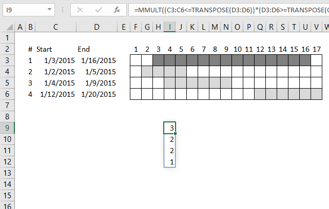
The image above shows date ranges in cell range D3:E7, the condition is in cell H2. The condition is matched to cell range C3:C7.
Row 9 shows dates from 1/1/2010 to 1/27/2010. Row 10 shows date range #1 across dates. Row 11 shows date range #2. Date range #3 is not highlighted, it does not match the condition specified in cell H2. The formula is ignoring this date range.
Row 13 shows date range #4 and date range #5 is not overlapping any date range at all.
The calendar makes it easy to spot the earliest and latest overlapping date, this will make it easy to verify the outcome of the formula.
I want to identify the overlap based on criteria but now I want to know what is that min date and the max date. Any tricks up your sleeve?
The following formulas calculates the min and max date from overlapping date ranges:
Array formula in cell H3:
Array formula in cell H4:
I recommend Excel Tables, they allow you to add and delete date ranges without the need to adjust cell references in the above formulas. References to Excel Tables are called "structured references" and they look differently than regular cell references.
Here is an structured reference example: Table1[Category] It is a reference to data in column Category in Excel Table named Table1. It begins with the Excel Table name and then a beginning bracket, the column header name and an ending bracket.
Explaining array formula in cell H3
Step 1 - Create an array from 0 (zero) to n
This step creates numbers from 0 (zero) to n that we will use, in the next step, to create all dates between the earliest date and the latest date based on the date ranges we are working with.
The MAX function calculates the largest (latest) date from dates in column End: in Excel Table named Table1
MAX(Table1[End:])
becomes
MAX({40181; 40187; 40180; 40207; 40238})
and returns 40238.
The MIN function returns the smallest number from column Start: in Excel Table Table1.
MIN(Table1[Start:])
becomes
MIN({40179;40180;40179;40186;40235})
and returns 40179.
The INDEX function returns a cell reference based on the number of days there are between the earliest date and the latest date.
INDEX($1:$1, MAX(Table1[End:])-MIN(Table1[Start:])+1)
becomes
INDEX($1:$1, 40238-40179+1)
becomes
INDEX($1:$1, 59+1)
becomes
INDEX($1:$1, 60)
returns cell reference BH1.
The colon character allows you to concatenate two cell references.
$A$1:INDEX($1:$1, MAX(Table1[End:])-MIN(Table1[Start:])+1))
becomes
$A$1:BH1
The column function calculates the column numbers from each cell in cell range $A$1:BH1.
COLUMN($A$1:INDEX($1:$1, MAX(Table1[End:])-MIN(Table1[Start:])+1))
becomes
COLUMN($A$1:BH1)
and returns
{1, 2, 3, 4, 5, 6, 7, 8, 9, 10, 11, 12, 13, 14, 15, 16, 17, 18, 19, 20, 21, 22, 23, 24, 25, 26, 27, 28, 29, 30, 31, 32, 33, 34, 35, 36, 37, 38, 39, 40, 41, 42, 43, 44, 45, 46, 47, 48, 49, 50, 51, 52, 53, 54, 55, 56, 57, 58, 59, 60}
Step 2 - Calculate dates
If we add array of numbers, calculated in the previous step, to a date we get an array of dates.
MIN(Table1[Start:])+COLUMN($A$1:INDEX($1:$1, MAX(Table1[End:])-MIN(Table1[Start:])+1))-1
becomes
MIN(Table1[Start:])+{1, 2, 3, 4, 5, 6, 7, 8, 9, 10, 11, 12, 13, 14, 15, 16, 17, 18, 19, 20, 21, 22, 23, 24, 25, 26, 27, 28, 29, 30, 31, 32, 33, 34, 35, 36, 37, 38, 39, 40, 41, 42, 43, 44, 45, 46, 47, 48, 49, 50, 51, 52, 53, 54, 55, 56, 57, 58, 59, 60}-1
becomes
MIN(Table1[Start:])+{0, 1, 2, 3, 4, 5, 6, 7, 8, 9, 10, 11, 12, 13, 14, 15, 16, 17, 18, 19, 20, 21, 22, 23, 24, 25, 26, 27, 28, 29, 30, 31, 32, 33, 34, 35, 36, 37, 38, 39, 40, 41, 42, 43, 44, 45, 46, 47, 48, 49, 50, 51, 52, 53, 54, 55, 56, 57, 58, 59}
and returns
{40179, 40180, 40181, 40182, 40183, 40184, 40185, 40186, 40187, 40188, 40189, 40190, 40191, 40192, 40193, 40194, 40195, 40196, 40197, 40198, 40199, 40200, 40201, 40202, 40203, 40204, 40205, 40206, 40207, 40208, 40209, 40210, 40211, 40212, 40213, 40214, 40215, 40216, 40217, 40218, 40219, 40220, 40221, 40222, 40223, 40224, 40225, 40226, 40227, 40228, 40229, 40230, 40231, 40232, 40233, 40234, 40235, 40236, 40237, 40238}
We will be using this array of dates to check which dates overlap each other.
Step 3 - Compare date array to start dates
MIN(Table1[Start:])+COLUMN($A$1:INDEX($1:$1, MAX(Table1[End:])-MIN(Table1[Start:])+1))-1>=Table1[Start:]
becomes
{40179, 40180, 40181, 40182, 40183, 40184, 40185, 40186, 40187, 40188, 40189, 40190, 40191, 40192, 40193, 40194, 40195, 40196, 40197, 40198, 40199, 40200, 40201, 40202, 40203, 40204, 40205, 40206, 40207, 40208, 40209, 40210, 40211, 40212, 40213, 40214, 40215, 40216, 40217, 40218, 40219, 40220, 40221, 40222, 40223, 40224, 40225, 40226, 40227, 40228, 40229, 40230, 40231, 40232, 40233, 40234, 40235, 40236, 40237, 40238}>=Table1[Start:]
becomes
{40179, 40180, 40181, 40182, 40183, 40184, 40185, 40186, 40187, 40188, 40189, 40190, 40191, 40192, 40193, 40194, 40195, 40196, 40197, 40198, 40199, 40200, 40201, 40202, 40203, 40204, 40205, 40206, 40207, 40208, 40209, 40210, 40211, 40212, 40213, 40214, 40215, 40216, 40217, 40218, 40219, 40220, 40221, 40222, 40223, 40224, 40225, 40226, 40227, 40228, 40229, 40230, 40231, 40232, 40233, 40234, 40235, 40236, 40237, 40238}>={40179; 40180; 40179; 40186; 40235}
and returns {TRUE, TRUE, TRUE, ... , TRUE}
This array is shortened for obvious reasons.
Step 5 - Compare date array to end dates
(MIN(Table1[Start:])+COLUMN($A$1:INDEX($1:$1, MAX(Table1[End:])-MIN(Table1[Start:])+1))-1)<=Table1[End:])
returns {TRUE, TRUE, TRUE, ... ,TRUE}.
Step 6 - Multiply arrays
We want both conditions to be met, in order to do that we must multiply the arrays (AND logic)
(MIN(Table1[Start:])+COLUMN($A$1:INDEX($1:$1, MAX(Table1[End:])-MIN(Table1[Start:])+1))-1>=Table1[Start:])*((MIN(Table1[Start:])+COLUMN($A$1:INDEX($1:$1, MAX(Table1[End:])-MIN(Table1[Start:])+1))-1)<=Table1[End:])
becomes
{TRUE, TRUE, TRUE, ... , TRUE} * {TRUE, TRUE, TRUE, ... , TRUE}
and returns {1, 1, 1, ... , 1}.
The equivalent value of boolean value TRUE is 1 and FALSE is 0 (zero). Excel converts the boolean values when you perform arithmetic operations.
Step 7 - Calculate which rows meet the condition
The equal sign allows you to compare a value to a value or in this case an array of values to a value.
(Table1[Category]=$H$2)
becomes
{"A";"A";"B";"A";"C"}="A"
and returns {TRUE; TRUE; FALSE; TRUE; FALSE}.
Step 6 - Multiply arrays
(Table1[Category]=$H$2)*(MIN(Table1[Start:])+COLUMN($A$1:INDEX($1:$1, MAX(Table1[End:])-MIN(Table1[Start:])+1))-1>=Table1[Start:])*((MIN(Table1[Start:])+COLUMN($A$1:INDEX($1:$1, MAX(Table1[End:])-MIN(Table1[Start:])+1))-1)<=Table1[End:])
becomes
{TRUE; TRUE; FALSE; TRUE; FALSE} * {1, 1, 1, ... , 1}
and returns {1, 1, 1, ... , 0}.
Keep in mind that a semicolon separates values row-wise and commas respectively column-wise.
Step 7 - Create an array of 1's.
The power of character ^ converts all dates in Table column Start: to 1.
Table1[Start:]^0
becomes
{1; 1; 1; 1; 1}
The transpose function allows you to convert a vertical range to a horizontal range, or vice versa.
TRANSPOSE(Table1[Start:]^0)
becomes
TRANSPOSE({1; 1; 1; 1; 1})
and returns {1, 1, 1, 1, 1}.
Step 8 - Add values vertically
MMULT(TRANSPOSE(Table1[Start:]^0), (Table1[Category]=$H$2)*(MIN(Table1[Start:])+COLUMN($A$1:INDEX($1:$1, MAX(Table1[End:])-MIN(Table1[Start:])+1))-1>=Table1[Start:])*((MIN(Table1[Start:])+COLUMN($A$1:INDEX($1:$1, MAX(Table1[End:])-MIN(Table1[Start:])+1))-1)<=Table1[End:]))
becomes
MMULT({1, 1, 1, 1, 1}, (Table1[Category]=$H$2)*(MIN(Table1[Start:])+COLUMN($A$1:INDEX($1:$1, MAX(Table1[End:])-MIN(Table1[Start:])+1))-1>=Table1[Start:])*((MIN(Table1[Start:])+COLUMN($A$1:INDEX($1:$1, MAX(Table1[End:])-MIN(Table1[Start:])+1))-1)<=Table1[End:]))
becomes
MMULT({1, 1, 1, 1, 1}, {1, 1, 1, ... , 1})
and returns {1, 2, 2, ... , 0}.
Step 9 - Check if value is above 1
A number above 1 indicates it is an overlapping date. The position of each number in the array corresponds to date in the date array. We can use this to extract the overlapping dates in the next step.
MMULT(TRANSPOSE(Table1[Start:]^0), (Table1[Category]=$H$2)*(MIN(Table1[Start:])+COLUMN($A$1:INDEX($1:$1, MAX(Table1[End:])-MIN(Table1[Start:])+1))-1>=Table1[Start:])*((MIN(Table1[Start:])+COLUMN($A$1:INDEX($1:$1, MAX(Table1[End:])-MIN(Table1[Start:])+1))-1)<=Table1[End:]))>1
becomes
{1, 2, 2, ... , 0}>1
and returns {FALSE, TRUE, TRUE, ... , FALSE}
Step 10 - Convert boolean values to corresponding dates
The IF function determines if a date will be returned or nothing "" based on the logical expression.
IF(MMULT(TRANSPOSE(Table1[Start:]^0), (Table1[Category]=$H$2)*(MIN(Table1[Start:])+COLUMN($A$1:INDEX($1:$1, MAX(Table1[End:])-MIN(Table1[Start:])+1))-1>=Table1[Start:])*((MIN(Table1[Start:])+COLUMN($A$1:INDEX($1:$1, MAX(Table1[End:])-MIN(Table1[Start:])+1))-1)<=Table1[End:]))>1, MIN(Start)+COLUMN($A$1:INDEX($1:$1, 0, MAX(Table1[End:])-MIN(Table1[Start:])+1))-1, "")
becomes
IF({FALSE, TRUE, TRUE, ... , FALSE}, MIN(Start)+COLUMN($A$1:INDEX($1:$1, 0, MAX(Table1[End:])-MIN(Table1[Start:])+1))-1, "")
becomes
IF({FALSE, TRUE, TRUE, ... , FALSE}, {40179, 40180, 40181, ... , 40238}, "")
and returns
{"", 40180, 40181, ... , "}.
Step 11 - Extract the latest date
The MAX function returns the largest date from the array ignoring blanks.
MAX(IF(MMULT(TRANSPOSE(Table1[Start:]^0), (Table1[Category]=$H$2)*(MIN(Table1[Start:])+COLUMN($A$1:INDEX($1:$1, MAX(Table1[End:])-MIN(Table1[Start:])+1))-1>=Table1[Start:])*((MIN(Table1[Start:])+COLUMN($A$1:INDEX($1:$1, MAX(Table1[End:])-MIN(Table1[Start:])+1))-1)<=Table1[End:]))>1,MIN(Start)+COLUMN($A$1:INDEX($1:$1,0,MAX(Table1[End:])-MIN(Table1[Start:])+1))-1,""))
becomes
MAX({"", 40180, 40181, ... , "})
and returns 40187 (1/9/2010).
Overlapping category
This article demonstrates formulas that calculate the number of overlapping ranges for all ranges, finds the most overlapped range and […]
Excel categories
41 Responses to “Identify rows of overlapping records”
Leave a Reply
How to comment
How to add a formula to your comment
<code>Insert your formula here.</code>
Convert less than and larger than signs
Use html character entities instead of less than and larger than signs.
< becomes < and > becomes >
How to add VBA code to your comment
[vb 1="vbnet" language=","]
Put your VBA code here.
[/vb]
How to add a picture to your comment:
Upload picture to postimage.org or imgur
Paste image link to your comment.
Chandoo has posted a much shorter better formula: https://chandoo.org/wp/2010/06/01/date-overlap-formulas/
Oscar, could you explain the COUNT($B$6:$B$12)-1 bit in the formula...
Peter,
Here is a shorter formula: =SUMPRODUCT((C6<=$D$6:$D$12)*(D6>=$C$6:$C$12)*(ROW(C6)<>ROW($C$6:$C$12)))>0. Copy cell and paste it down as far as needed.
The formula returns TRUE if overlapping.
Peter,
=SUMPRODUCT((C6< =$D$6:$D$12)*(D6>=$C$6:$C$12))>1 is shorter.
Copy cell and paste it down as far as needed.
The formula returns TRUE if overlapping.
Thanks Oscar...... appreciate your prompt feedback
Hey Oscar,
I tried this and I can't get accurate results with the data set I'm working with.
As an example, how would the formula work if I wanted to find the overlap between the start 2/end 2 dates versus start 1/end 1 dates?
Title - Start 1 End 1 Start 2 End 2 Overlap?
Titans 6/1/14 5/31/15 6/1/14 6/30/14
Titans 6/1/16 5/31/17 8/1/14 8/31/14
Titans 6/1/18 5/31/19 6/1/17 5/31/18
Titans 7/1/21 6/30/23 6/1/19 2/29/20
In the above example, in the "overlap" cell, it should say "yes" for row 1 and row 2, and "no" for row 3 and row 4.
Thanks so much for the help!
Brett
Brett,
read this:
Find overlapping date ranges with criterion
Hi Oscar,
Oh my, this is so close, but is just shy of solving the problem.
The problem I'm encountering if is there are multiple "titles".
In the example below, the formula has to find a match in the "title" column and then look at all start and end dates for the matched title to see if there is any cross over.
Here's another example:
Name Start 1 End 1 Start 2 End 2 Overlap?
Titans 6/1/14 5/31/15 6/1/14 6/30/14 TRUE
Titans 6/1/16 5/31/17 8/1/14 8/31/14 TRUE
Titans 6/1/18 5/31/19 6/1/17 5/31/18 FALSE
Titans 7/1/21 6/30/23 6/1/19 2/29/20 FALSE
Campers 10/1/15 9/30/16 10/1/14 9/30/15
Campers 10/1/17 9/30/18 9/1/16 9/30/17
Campers 11/1/21 4/30/22 10/1/17 6/30/20
Dark Horse 6/1/16 11/30/16 12/1/14 11/30/15
Dark Horse 12/1/16 11/30/17 12/1/15 5/31/16
Dark Horse 12/1/18 11/30/19 12/1/16 11/30/18
Gang 4/1/17 3/31/18 4/1/15 3/31/16
Gang 4/1/18 3/31/19 4/1/16 4/30/18
Ants 2/1/17 1/31/18 #N/A #N/A
Ants 2/1/19 1/31/20 #N/A #N/A
Again, this is way out of my league and thanks so much for putting your excel expertise to work!
Brett
Brett,
I am not sure I am following, what is the desired outcome in column F?
Hi Oscar,
When I copy (or auto fill) in the formula down in row F, it doesn't calculate the way your example does above and (except for rows 2 and 3), my results are "false" for rows 4 through 13.
Since this is an array formula, is there a special way I have to to copy the formula.
Or, can you post the excel version of your example above so I can look at the formula?
Thanks!
Brett
Brett,
expand the cell references to this:
=SUMPRODUCT((A2=$A$2:$A$13)*((B2<=$E$2:$E$13)*(C2>=$D$2:$D$13)+(D2<=$C$2:$C$13)*(E2>=$B$2:$B$13)))>0
Hi again,
I should also add that my data contains unique "titles" and my goal is for the formula to look at the differing start and end dates for each like title.
Thanks!
Brett
hi brett did u get the answer for your question as i am having similar trouble
Hi Oscar ,
I have similar problem as brett. I also want to check only for that ranges which have similar value for titles. Basically I want to compare overlapping only for those rows which have same value of say column1
Puneet,
Conditional formatting formula:
=SUMPRODUCT(($A2=$A$2:$A$9)*($B2<=$C$2:$C$9)*($C2>=$B$2:$B$9))>1
Good stuff Oscar!
I have a slightly different situation like Puneet's where I have 2 arbitrary reporting dates which I want to apply to a data set like the one you have there. But instead of returning TRUE/FALSE, I need to return the total count of days from the data set which fall between the 2 reporting dates. The output needs to be 1 value, rather than one per row. Struggling to get my head around this!
TC,
Is this what you are looking for?
Hi Oscar, This is really helpful and hoping you can help. My issue is the same as Puneet's in which I do want to identify the overlap based on a criteria but now I want to know what is that min date and the max date. Any tricks up your sleeve?
Thank you!
Liz,
read this post:
Calculate min and max date among overlapping date ranges and based on a condition
Hi Oscar,
Thank you for your post on the min and max. I've been using your formulas but I don't think it is working for the set of values that I'm working with since my dates include time.I have over 12000 records in my list and here is a snippet. Need to calculate the non-overlap hours per Identifier. How can I get to this?
Start End Identifier Non-Overlap Hours per Identifier
11/1/2012 0:00 11/1/2012 10:30 115854 10.5
11/1/2012 0:00 11/1/2012 10:30 117534 10.5
11/1/2012 1:00 11/1/2012 17:00 115854 6.5
11/1/2012 5:00 11/1/2012 15:00 117534 4.5
11/1/2012 10:00 11/1/2012 18:00 118929 8
11/1/2012 10:00 11/1/2012 18:00 118929 0
11/1/2012 14:00 11/1/2012 17:00 113569 3
11/1/2012 14:00 11/1/2012 17:00 113569 0
Using your formula I added an If statement so that if there is an overlap put a 0 and then put a 1 when there is no overlap but I do not think that addresses what I need to solve. Any suggestions are greatly appreciated.
Liz,
I am not following, isn´t the Non-Overlap Hours per Identifier 1 hour, in this example?
11/1/2012 0:00 11/1/2012 10:30 115854 10.5 <-- 1 hour and 11/1/2012 1:00 11/1/2012 17:00 115854 6.5
Hi Oscar,
I see what you mean now that the first one will be 1 hour. I need to calculate the total non-overlap hours per identifier.
I appreciate your help!
[…] Liz asks: […]
Thanks! Took a little tweaking, but this does just what I need.
For this, I use Sumproduct with two conditions:
1. Current start date = Start data range
mma173,
Can you tell us the formula?
Hi again Oscar!
On to Step 2!
The people using this file are not "Tech" savey, in fact they don't like Excel at all. So I'm trying to make it easier for them to use. The values in D6:F12 are understandable to me, however "Non-Tech Bob" comes and ask's, "How can this cell(D6) show a 9 when there are only 7 names?"
The easiest solution would be to insert a new column at the beginning of the file and starting in cell A6, enter the text "Line 1".
A7 "Line 2"
A8 "Line 3" and so on..
Is there a way for the formula in D6 (now E6) to return the text string in column A rather than the ROW number?
(New
Column)
A B C D E F G H
LINE # NAME: START DATE: END DATE: Overlapping with lines:
Line 1 Jeff 2010-01-04 2010-01-08 Line 4 Line 7
Line 2 Thomas 2010-01-11 2010-01-15
Line 3 Tim 2010-01-18 2010-01-22
Line 4 Shaun 2010-01-07 2010-01-09 Line 1
Line 5 Simon 2010-01-25 2010-01-29
Line 6 Theodor2010-02-01 2010-02-05
Line 7 John 2010-01-03 2010-01-04 Line 1
This way I could hide the "Row and Column" headers under Options and reduce the clutter on the page.
Thanks again for your assistance!
Boy did THAT not work!
This should help.
https://s11.postimg.org/jgjaowhqr/Identifying_Overlap_Ranges.png
cwrbelis,
Is there a way for the formula in D6 (now E6) to return the text string in column A rather than the ROW number?
Sure! There are two sheets in the workbook below.
Identify-overlapping-date-rangesv2.xlsx
Hello,
I am having a problem figuring out the below.
I have multiple identifiers and I need to find out if they have overlapping dates and times? Can someone please help? Thank you kindly.
Facilitator Date Time Overlap
Susannah Cahillane Tuesday, October 7, 2014 04:00 pm-07:00 pm
Emily Ferrara Tuesday, September 30, 2014 04:00 pm-07:00 pm
Lynette Bradley Thursday, October 2, 2014 04:00 pm-07:00 pm
Renata Pienkawa Thursday, December 4, 2014 04:00 pm-06:00 pm
Dana Furbush Thursday, October 2, 2014 03:30 pm-06:30 pm
Ariel Nelson Monday, November 17, 2014 03:30 pm-06:30 pm
Carla Bruzzese Thursday, October 2, 2014 04:00 pm-07:00 pm
Elizabeth Gospodarek Thursday, October 2, 2014 04:00 pm-07:00 pm
Sunita Mehrotra Monday, September 22, 2014 04:00 pm-07:00 pm
Kellie Jones Thursday, October 9, 2014 04:30 pm-07:30 pm
Pavlina Gatikova Tuesday, October 7, 2014 04:00 pm-06:00 pm
Gail Arsenault Monday, October 6, 2014 03:45 pm-06:45 pm
Sunita Mehrotra Wednesday, October 1, 2014 04:30 pm-07:30 pm
Sunita Mehrotra Tuesday, October 7, 2014 04:30 pm-07:30 pm
Christine Nicholson Wednesday, October 1, 2014 04:30 pm-06:30 pm
Allison Levit Monday, October 27, 2014 03:30 pm-06:30 pm
Peter Dillon Wednesday, October 1, 2014 04:00 pm-07:00 pm
Great post! Here's a solution, which uses a couple of (changeable) assumptions:
=SUMPRODUCT(FREQUENCY(ROW(INDIRECT("A"&HOUR(A7)+ 1&":A"&HOUR(B7))), HOUR(C2:C3)), D2:D4)
By quantizing the time (into hours in this case), and then counting the quantity in each rate bucket, we can then do a SUMPRODUCT against the rates. Remember that the FREQUENCY function returns one more item than the number of buckets passed to it, so I left out the final bucket time to compensate.
-Alex
Alex,
fantastic, why didn´t I think of that.
Thank you for your valuable comment!
I'm willing to take my medicine if there's something simple in here that I should have seen, but here goes...
How do I find overlapping ranges (using the MEDIAN function) for three to six time ranges? Or do I have to figure each range separately, then combine it into one IF statement using AND statements?
Forgot to add something to my previous post:
There are a variable number of time range(s) within each day - anywhere from 0 to 4 time ranges - and the number of ranges may change from day to day. Any formula must be able to handle this.
Henry Dishington,
Do you want to find overlapping ranges? Read this:
https://www.get-digital-help.com/identify-overlapping-records/
Or do you want to count overlapping days?
Another solution at your quest, with CSE formula:B2:B4,$A$7,B2:B4)>0,IF($B$7B2:B4,$A$7,B2:B4),0)*D2:D4*24)
=SUM(IF(IF($B$7
for some unknown reason, previous paste was an error.
Correct formula is:
{=SUM(IF(IF($B$7A2:A4,$A$7,A2:A4)>0,IF($B$7A2:A4,$A$7,A2:A4),0)*C2:C4*24)}
O, no, not again!
I try to upload a file.
Hi Oscar,
Thank you for this wonderful resource you've created here.
I was able to use your formula to identify overlapping dates, however, I have to sum values from a column based upon overlapping dates.
In the example below I have a set of allowances provided by a coffee vendor for one of their products. I would need to have excel add $5.04 to $1.26 because the second row allowance overlaps with the first row's dates and then have this logic applied throughout the table. Multiple allowances can be summed if there are multiple date overlaps. Might you be able to show how I could have excel sum the allowances and maybe even identify the exact dates that are overlapping?
I have referenced your other pages on accounting for overlapping dates over multiple ranges, but I am afraid that setting up a matrix will not prove practical when the dates span over several months and we may be querying thousands of rows at one time.
ITEM_DESCRIP ALLOW_DATE_EFF ALLOW_DATE_EXP ALLOW_AMT ALLOW_TYPE OVERLAPPING?
CAMERONS DECAF BREAKFAST BLEND 10 OZ 2/24/2020 3/23/2020 $5.04 PA TRUE
CAMERONS DECAF BREAKFAST BLEND 10 OZ 3/1/2020 3/16/2020 $1.26 PA TRUE
CAMERONS DECAF BREAKFAST BLEND 10 OZ 3/22/2020 4/20/2020 $1.26 PA TRUE
CAMERONS DECAF BREAKFAST BLEND 10 OZ 3/23/2020 4/20/2020 $5.04 PA TRUE
CAMERONS DECAF BREAKFAST BLEND 10 OZ 4/20/2020 5/18/2020 $5.04 PA TRUE
CAMERONS DECAF BREAKFAST BLEND 10 OZ 5/18/2020 6/15/2020 $5.04 PA TRUE
CAMERONS DECAF BREAKFAST BLEND 10 OZ 6/15/2020 7/13/2020 $5.04 PA TRUE
Hi Oscar,
Thanx for your answers. I have slightly different problem and I cant find solution.
I am trying to calculate how many calls overlap at my call center at one time, so I can better plan shifts. I am using this formula:
=SUMPRODUCT(--((C2+O2=$C$2:$C$11870+$O$2:$O$11870)=0))
However, I would like to know number of overlaped calls, when the overlap is longer than, lets say 10seconds.
Can you help please.
Thanx Milos