Search for a sequence of values
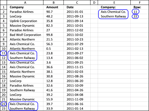
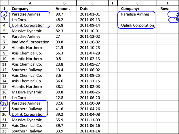
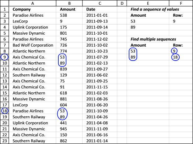
This article demonstrates array formulas that identify two search values in a row or in a sequence. The image above shows two search values in cell E2 and E3, the formula in cell F2 looks for those search values in column A and the corresponding row numbers are returned if they match.
The order is important, meaning the search values must be in a sequence exactly as they are written in cell E2 and E3.
Table of Contents
- How to find two search values next to each other vertically?
- How to find all instances of two search values next to each other vertically?
- How to find a sequence with any value between?
- Find multiple sequences with any value between?
- Get Excel file
- How to calculate the first row number of two cells containing search values next to each other vertically?
- How to calculate row numbers of two cells containing search values next to each other vertically?
- Lookup for a multi-level sequence
- Lookup for multiple multi-level sequences
- Wildcard search for a sequence
- Wildcard search for multiple sequences
- Get Excel file
1. How to find two search values next to each other vertically?
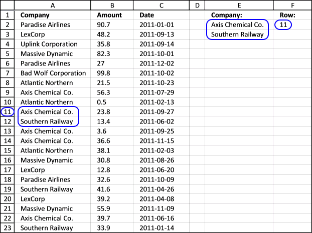
The image above shows a formula in cell F2 that returns only the first match based on the search values in cell E2 and E3.
This array formula finds the sequence "Axis Chemical Co." (cell E2) and "Southern Railway" (cell E3) in two consecutive cells in column A and returns the row number in cell F2.
Array formula in cell F11:
Update 3-17-2021, the following Excel 365 formula extracts the corresponding values from the column B and C based on the found sequences:
How to use the FILTER function
How to enter an array formula
There is no need to enter the formulas if you own Excel 365, it uses dynamic array formulas.
- Double press with left mouse button on cell F2. The prompt shows up.
- Paste formula to cell.
- Press and hold CTRL + SHIFT simultaneously.
- Press Enter once.
- Release all keys.
The formula now looks like this: {=MATCH(E2&E3, $A$1:$A$23&$A$2:$A$24, 0)}
Don't enter the beginning and ending curly brackets yourself, they appear automatically if you managed to enter the array formula successfully.
Explaining formula in cell F2
Step 1 - Concatenate cells
The ampersand lets you concatenate cell values.
E2&E3
returns "Axis Chemical Co.Southern Railway"
Step 2 - Concatenate cell ranges
The second argument in the MATCH function is $A$1:$A$23&$A$2:$A$24. The ampersand concatenates the two cell ranges into one. By concatenating a value with the value below you can easily search for a sequence of values.
$A$1:$A$23&$A$2:$A$24
returns {"CompanyParadise Airlines";... ;"Southern Railway"}
Step 3 - Find the relative position
The MATCH function returns the relative position of an item in an array or cell reference that matches a specified value in a specific order.
MATCH(lookup_value, lookup_array, [match_type])
MATCH(E2&E3, $A$1:$A$23&$A$2:$A$24, 0)
becomes
MATCH("Axis Chemical Co.Southern Railway", {"CompanyParadise Airlines";... ;"Southern Railway"}, 0)
and returns 11.
2. How to find all instances of two search values next to each other vertically?
The image above demonstrates an array formula that returns row numbers of all found sequences based on the search values in cells E2 and E3.
Array formula in cell F2:
Copy cell F2 and paste cells below as far as needed.
Update 3-17-2021,the following Excel 365 formula extracts the corresponding values from the column B and C based on the found sequences:
How to use the FILTER function
Explaining formula in cell F2
Step 1 - Logical expression
$E$2&$E$3=$A$1:$A$23&$A$2:$A$24
becomes
returns {FALSE; FALSE; ... ; FALSE}
Step 2 - Create a sequence of numbers from 1 to n
The MATCH function returns the relative position of an item in an array or cell reference that matches a specified value in a specific order.
MATCH(lookup_value, lookup_array, [match_type])
MATCH(ROW($A$2:$A$23), ROW($A$2:$A$23)))
returns {1; 2; ... ; 22}
Step 3 - Evaluate IF function
The IF function returns the corresponding row number if the logical value is TRUE and FALSE if FALSE.
IF($E$2&$E$3=$A$1:$A$23&$A$2:$A$24, MATCH(ROW($A$2:$A$23), ROW($A$2:$A$23)))
returns {FALSE; FALSE; ... ; 22; FALSE}
Step 4 - Find k-th smallest number in array
The SMALL function returns the k-th smallest value from a group of numbers. It ignores text and boolean values.
SMALL(array, k)
SMALL(IF($E$2&$E$3=$A$1:$A$23&$A$2:$A$24, MATCH(ROW($A$2:$A$23), ROW($A$2:$A$23))), ROWS($A$1:A1))
and returns 11.
3. How to find a sequence with any value between?
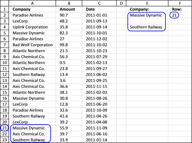
The image above demonstrates a formula in cell F2 that looks for a sequence of three values where the middle one can be anything.
Array formula in cell F2:
Update 3-17-2021, the following Excel 365 formula extracts the corresponding values from the column B and C based on the found sequences:
Explaining formula in cell F2
Step 1 - Concatenate lookup_value
Note that cells E2 and E4 are now being concatenated.
E2&E4
becomes
"Massive Dynamic"&"Southern Railway"
and returns
"Massive DynamicSouthern Railway"
Step 2 - Concatenate lookup_array
The lookup array consists of two cell ranges concatenated, note that the first one begins at $A$1 and the second one at cell $A$3.
$A$1:$A$23&$A$3:$A$25
returns
{"CompanyLexCorp";... ;"Southern Railway"}
Step 3 - Find the relative position of the lookup_value in the lookup_array
The MATCH function returns the relative position of an item in an array or cell reference that matches a specified value in a specific order.
MATCH(lookup_value, lookup_array, [match_type])
MATCH(E2&E4,$A$1:$A$23&$A$3:$A$25,0)
returns 21.
If you examine this combined cell ref $A$1:$A$23&$A$3:$A$25 you can see that the first one starts at A1 and the second one at A3. This is because the second value in the sequence is a value that can be anything. Let us see the values behind these cell refs.
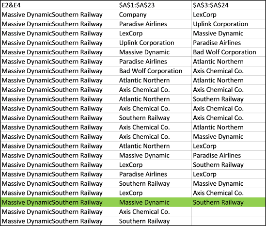
Cell reference $A$3:$A$24 is wrong in the image above, it should be $A$3:$A$25.
Find multiple sequences with any value between
Array formula in cell F2:
Update 3-17-2021, the following Excel 365 formula extracts the corresponding values from the column B and C based on the found sequences:
Finding a sequence - potential problems
Array formula in cell F2:
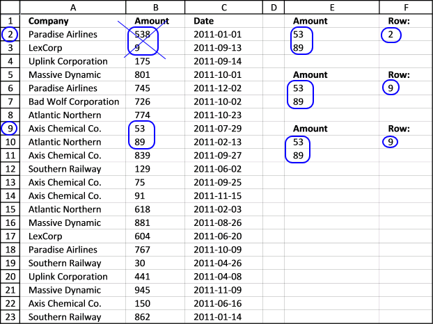
As you can see, the formula returns row 2. Why is that? The MATCH function looks for the value in cell E2 and E3 combined like this, 53 and 89 becomes 5389. The values in cell B2 and B3 are 538 and 9, becomes 5389 and that is a match.
So if we add a delimiting character we can rule out these problems, see the next formula.
Array formula in cell F6:
But to be really sure that this works you must check that the character "-" does not exist at all in column B or you could get same the error again. The next formula uses the COUNTIFS function and I think this is the best method, no need for delimiting characters.
Array formula in cell F10:
The downside with this formula is that you can´t find multiple sequences in a column.
If you want to learn more about array formulas join Advanced excel course.
Read more
- Find a sequence of values - wildcard search
- Repeat values
- Create number sequences
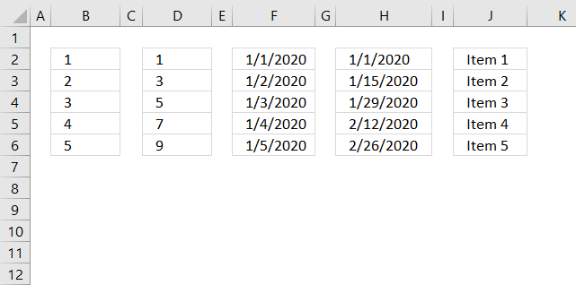
- Merge lists with criteria
6. How to calculate the first row number of two cells containing search values next to each other vertically?
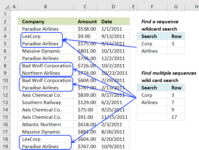
This section demonstrates array formulas that perform a wildcard search based on a sequence of values. The formulas return the row number of cells that contain the search values in a consecutive order.
The array formula in cell F3 returns the row number of the first two cells that contain the given search values.
Array formula in cell F3:
How to enter an array formula
To enter an array formula, type the formula in a cell then press and hold CTRL + SHIFT simultaneously, now press Enter once. Release all keys.
The formula bar now shows the formula with a beginning and ending curly bracket telling you that you entered the formula successfully. Don't enter the curly brackets yourself.
Explaining formula in cell F3
Step 1 - Create an array that shows where the specific sequence is
The COUNTIFS function lets you count values based on multiple conditions, in this case, I am also changing the cell references.
The first two arguments check for the value in cell E3 in cell range B1:B23. The third and fourth argument looks for the value in cell E4 in cell range B2:B24, note that the cell range in argument 4 relative the 2nd argument is offset by 1.
This cell reference technique lets you find values in a given sequence.
COUNTIFS(E3,B1:B23,E4,B2:B24) returns {0; 0; 0; 0; 0; 0; 0; 0; 1; 0; 0; 0; 0; 0; 0; 0; 0; 1; 0; 0; 0; 0; 0}.
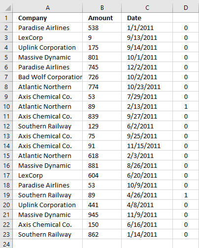
The array is shown in column D.
Step 2 - Find the relative position in the array
The MATCH function finds the position in the array based on a given value, if multiple values exist the position of the first is returned.
MATCH(1, COUNTIFS(E3, B1:B23, E4, B2:B24), 0)
becomes
MATCH(1, {0; 0; 0; 0; 0; 0; 0; 0; 1; 0; 0; 0; 0; 0; 0; 0; 0; 1; 0; 0; 0; 0; 0}, 0)
and returns 9 in cell F3.
7. How to calculate all row numbers of two cells containing search values next to each other vertically?
What I didn't show you was how to find multiple sequences with this particular array formula.
This array formula finds all instances of cells containing a sequence of values, the order is important. It returns their starting row number.
Array formula in cell F8:
Update 3-17-2021, the following Excel 365 formula extracts the corresponding row numbers from the found sequences:
Explaining formula in cell F8
See step 1 in the explanation above before reading the rest below.
Step 2 - Convert boolean value TRUE to row number in the array
The IF function uses a logical expression in the first argument to determine if the second or third argument is being returned. The second argument if the logical expression evaluates to TRUE and the third argument if the logical expression evaluates to FALSE.
IF(COUNTIFS($E$8, $B$1:$B$23, $E$9, $B$2:$B$24)=1, MATCH(ROW($A$1:$A$23), ROW($A$1:$A$23)), "")
becomes
IF({0; 0; 0; 0; 0; 0; 0; 0; 1; 0; 0; 0; 0; 0; 0; 0; 0; 1; 0; 0; 0; 0; 0}, MATCH(ROW($A$1:$A$23), ROW($A$1:$A$23)), "")
becomes
IF({0; 0; 0; 0; 0; 0; 0; 0; 1; 0; 0; 0; 0; 0; 0; 0; 0; 1; 0; 0; 0; 0; 0}, {1; 2; 3; 4; 5; 6; 7; 8; 9; 10; 11; 12; 13; 14; 15; 16; 17; 18; 19; 20; 21; 22; 23}, "")
and returns
{"";"";"";"";"";"";"";"";9;"";"";"";"";"";"";"";"";18;"";"";"";"";""}
Step 3 - Extract row numbers sorted smallest to largest
The SMALL function extracts the k-th smallest number in array, it ignores blanks.
SMALL(IF(COUNTIFS($E$8, $B$1:$B$23, $E$9, $B$2:$B$24)=1, MATCH(ROW($A$1:$A$23), ROW($A$1:$A$23)), ""), ROW(A1))
becomes
SMALL({"";"";"";"";"";"";"";"";9;"";"";"";"";"";"";"";"";18;"";"";"";"";""}, ROW(A1))
The ROW function returns the row number based on a cell reference, this cell reference is relative meaning it will change as the formula is copied to cells below. This makes the formula extracting a new value in each cell.
SMALL({"";"";"";"";"";"";"";"";9;"";"";"";"";"";"";"";"";18;"";"";"";"";""}, ROW(A1))
becomes
SMALL({"";"";"";"";"";"";"";"";9;"";"";"";"";"";"";"";"";18;"";"";"";"";""}, 1)
returns 9 in cell F8.
8. Lookup for a multi-level sequence
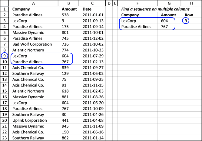
The next array formula looks for consecutive values in columns and rows. This means that the values in cell range F3:G4 must be found in column A and B in order to return the corresponding row number.
Array formula in cell H3:
Use this formula if you are looking for the first instance of a sequence. It looks for a specific sequence (LexCorp and Paradise Airlines) in column A and for 604 and 767 in column B. LexCorp and 604 must be on the same row and Paradise Airlines and 767 must be on the next row below.
Update 3-17-2021, the following Excel 365 formula extracts the corresponding dates in column C from the found sequences:
Explaining formula in cell H3
Step 1 - Create an array that shows where the specific sequence is
The COUNTIFS function lets you count values based on multiple conditions, in this case, I am also doing changes to the cell references.
COUNTIFS(F3, A1:A23, F4,A2:A24, G3, B1:B23, G4, B2:B24) returns {0; 0; 0; 0; 0; 0; 0; 0; 1; 0; 0; 0; 0; 0; 0; 0; 1; 0; 0; 0; 0; 0; 0}.
The second record (cell F4 and G4) are offset 1 row in order to find two consecutive records.
Step 2 - Find the relative position in the array
The MATCH function finds the position in the array based on a given value if multiple values exist the position of the first is returned.
MATCH(1, COUNTIFS(F3, A1:A23, F4,A2:A24, G3, B1:B23, G4, B2:B24), 0)
becomes
MATCH(1, {0; 0; 0; 0; 0; 0; 0; 0; 1; 0; 0; 0; 0; 0; 0; 0; 1; 0; 0; 0; 0; 0; 0}, 0)
and returns 9 in cell H3.
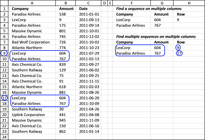
9. Lookup for multiple multi-level sequences
Array formula in cell H8:
It is like the formula above but it returns the location of multiple sequences.
Update 3-17-2021, the following Excel 365 formula extracts the corresponding dates in column C from the found sequences:
Explaining formula in cell H8
See step 1 in the explanation above before reading the rest below.
Step 2 - Convert boolean value TRUE to row number in array
The IF function uses a logical expression in the first argument to determine if the second or third argument is being returned. The second argument if the logical expression evaluates to TRUE and the third argument if the logical expression evaluates to FALSE.
IF(COUNTIFS($F$8, $A$1:$A$23, $F$9, $A$2:$A$24, $G$8, $B$1:$B$23, $G$9, $B$2:$B$24)=1, MATCH(ROW($A$1:$A$23), ROW($A$1:$A$23)), "")
becomes
IF({FALSE; FALSE; FALSE; FALSE; FALSE; FALSE; FALSE; FALSE; TRUE; FALSE; FALSE; FALSE; FALSE; FALSE; FALSE; FALSE; TRUE; FALSE; FALSE; FALSE; FALSE; FALSE; FALSE}, MATCH(ROW($A$1:$A$23), ROW($A$1:$A$23)), "")
becomes
IF({FALSE; FALSE; FALSE; FALSE; FALSE; FALSE; FALSE; FALSE; TRUE; FALSE; FALSE; FALSE; FALSE; FALSE; FALSE; FALSE; TRUE; FALSE; FALSE; FALSE; FALSE; FALSE; FALSE}, {1; 2; 3; 4; 5; 6; 7; 8; 9; 10; 11; 12; 13; 14; 15; 16; 17; 18; 19; 20; 21; 22; 23}, "")
and returns
{"";"";"";"";"";"";"";"";9;"";"";"";"";"";"";"";"";17;"";"";"";"";""}.
Step 3 - Extract row numbers sorted smallest to largest
The SMALL function extracts the k-th smallest number in array, it ignores blanks.
SMALL(IF(COUNTIFS($F$8, $A$1:$A$23, $F$9, $A$2:$A$24, $G$8, $B$1:$B$23, $G$9, $B$2:$B$24)=1, MATCH(ROW($A$1:$A$23), ROW($A$1:$A$23)), ""), ROW(A1))
becomes
SMALL({"";"";"";"";"";"";"";"";9;"";"";"";"";"";"";"";17;"";"";"";"";"";""}, ROW(A1))
The ROW function returns the row number based on a cell reference, this cell reference is relative meaning it will change as the formula is copied to cells below. This makes the formula extracting a new value in each cell.
SMALL({"";"";"";"";"";"";"";"";9;"";"";"";"";"";"";"";17;"";"";"";"";"";""}, ROW(A1))
becomes
SMALL({"";"";"";"";"";"";"";"";9;"";"";"";"";"";"";"";17;"";"";"";"";"";""}, 1)
returns 9 in cell F8.
10. Wild card search for a sequence
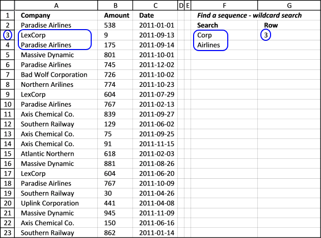
This demonstrates how to do a wild card search for a sequence. This formula returns the row number of the first found sequence in column A. The formula looks for a text string in a cell and another text string in the cell below. You don't need to enter the wild cards * (asterisks), see cell F3 and F4.
Update 3-17-2021, the following Excel 365 formula extracts the corresponding cell values in column B and C from all found sequences or consecutive values:
Explaining formula in cell G3
Step 1 - Find cells containing search value in cell F11
The FIND function returns the position of a specific string in another string, reading left to right. Note, the FIND function is case-sensitive.
FIND($F$11, $A$1:$A$23)
becomes
FIND("Corp",{"Company"; "Paradise Airlines"; "LexCorp"; "Paradise Airlines"; "Massive Dynamic"; "Paradise Airlines"; "Bad Wolf Corporation"; "Northern Airlines"; "Bad Wolf Corporation"; "Paradise Airlines"; "Axis Chemical Co."; "Southern Railway"; "Axis Chemical Co."; "Axis Chemical Co."; "Atlantic Northern"; "Massive Dynamic"; "LexCorp"; "Paradise Airlines"; "Southern Railway"; "Uplink Corporation"; "Massive Dynamic"; "Axis Chemical Co."; "Southern Railway"})
and returns {#VALUE!; #VALUE!; 4; #VALUE!; #VALUE!; #VALUE!; 10; #VALUE!; 10; #VALUE!; #VALUE!; #VALUE!; #VALUE!; #VALUE!; #VALUE!; #VALUE!; 4; #VALUE!; #VALUE!; 8; #VALUE!; #VALUE!; #VALUE!}.
Step 2 - Find cells containing search value in cell F12
FIND($F$12, $A$2:$A$24)
becomes
FIND("Airlines",{"Paradise Airlines"; "LexCorp"; "Paradise Airlines"; "Massive Dynamic"; "Paradise Airlines"; "Bad Wolf Corporation"; "Northern Airlines"; "Bad Wolf Corporation"; "Paradise Airlines"; "Axis Chemical Co."; "Southern Railway"; "Axis Chemical Co."; "Axis Chemical Co."; "Atlantic Northern"; "Massive Dynamic"; "LexCorp"; "Paradise Airlines"; "Southern Railway"; "Uplink Corporation"; "Massive Dynamic"; "Axis Chemical Co."; "Southern Railway"; 0})
and returns {10; #VALUE!; 10; #VALUE!; 10; #VALUE!; 10; #VALUE!; 10; #VALUE!; #VALUE!; #VALUE!; #VALUE!; #VALUE!; #VALUE!; #VALUE!; 10; #VALUE!; #VALUE!; #VALUE!; #VALUE!; #VALUE!; #VALUE!}
Step 3 - Multiply arrays
FIND($F$11, $A$1:$A$23)*FIND($F$12, $A$2:$A$24)
returns {#VALUE!; #VALUE!; 40; #VALUE!; #VALUE!; #VALUE!; 100; #VALUE!; 100; #VALUE!; #VALUE!; #VALUE!; #VALUE!; #VALUE!; #VALUE!; #VALUE!; 40; #VALUE!; #VALUE!; #VALUE!; #VALUE!; #VALUE!; #VALUE!}
Step 4 - Check if value is a number
ISNUMBER(FIND($F$11, $A$1:$A$23)*FIND($F$12, $A$2:$A$24))
becomes
ISNUMBER({#VALUE!; #VALUE!; 40; #VALUE!; #VALUE!; #VALUE!; 100; #VALUE!; 100; #VALUE!; #VALUE!; #VALUE!; #VALUE!; #VALUE!; #VALUE!; #VALUE!; 40; #VALUE!; #VALUE!; #VALUE!; #VALUE!; #VALUE!; #VALUE!})
and returns {FALSE; FALSE; TRUE; FALSE; FALSE; FALSE; TRUE; FALSE; TRUE; FALSE; FALSE; FALSE; FALSE; FALSE; FALSE; FALSE; TRUE; FALSE; FALSE; FALSE; FALSE; FALSE; FALSE}.
Step 5 - Find position of boolean value TRUE in array
The MATCH function finds the position in the array based on a given value, if multiple values exist the position of the first is returned.
MATCH(TRUE, ISNUMBER(FIND($F$11, $A$1:$A$23)*FIND($F$12, $A$2:$A$24)), 0)
becomes
MATCH(TRUE, {FALSE; FALSE; TRUE; FALSE; FALSE; FALSE; TRUE; FALSE; TRUE; FALSE; FALSE; FALSE; FALSE; FALSE; FALSE; FALSE; TRUE; FALSE; FALSE; FALSE; FALSE; FALSE; FALSE}, 0)
and returns 3.
11. Wild card search for multiple sequences
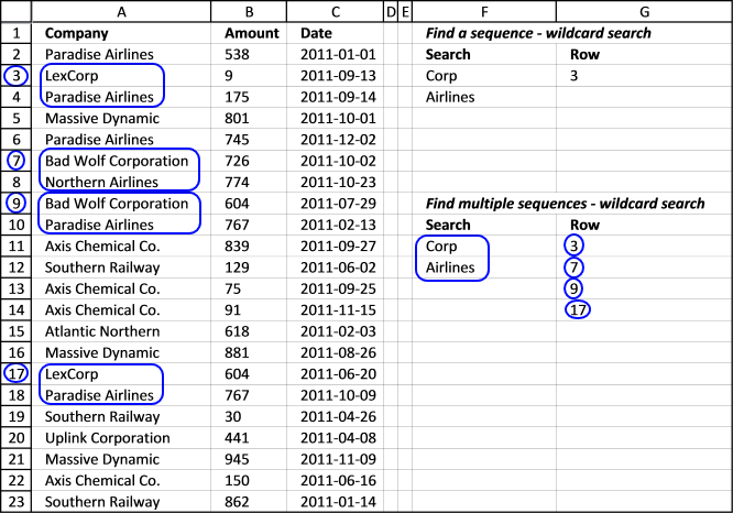
This demonstrates how to do wild card searches for multiple sequences. This formula returns the row number of all found sequences in column A. The sequence is in cell F11 and F12.
Array formula in cell G11:
If a cell contains "Corp" and the next cell beneath contains "Airlines" the array formula returns the row number.
12. Get Excel file
Sequence category
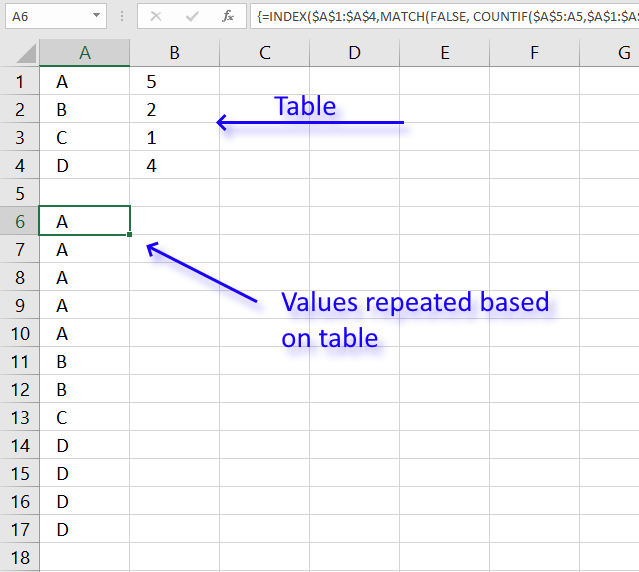
Table of Contents Repeat values Repeat the range according to criteria in loop Find the most/least consecutive repeated value […]
Excel has a great built-in tool for creating number series named Autofill. The tool is great, however, in some situations, […]
Excel categories
One Response to “Search for a sequence of values”
Leave a Reply
How to comment
How to add a formula to your comment
<code>Insert your formula here.</code>
Convert less than and larger than signs
Use html character entities instead of less than and larger than signs.
< becomes < and > becomes >
How to add VBA code to your comment
[vb 1="vbnet" language=","]
Put your VBA code here.
[/vb]
How to add a picture to your comment:
Upload picture to postimage.org or imgur
Paste image link to your comment.
Hi this is not working